1. Set Up
1.1 Introduction
This article is the third in a series comparing the fpp2, fpp3, and modeltime+timetk forecasting frameworks in R. It will focus on how to manually and automatically choose an ARIMA model for fitting various types of time series data. It will also show how to evaluate the residuals of a fitted model for white noise and how to minimize the AICc for model selection. The term ARIMA is short for AutoRegressive Integrated Moving Average.
1.2 Load Libraries
# Load libraries
library(fpp2)         # The forecasting OG
library(fpp3)         # The tidy version of fpp2
library(modeltime)    # The tidy forecasting newcomer
library(timetk)       # Companion to modeltime
library(parsnip)      # Common interface for specifying models
library(tidyverse)    # Data manipulation tools
library(rsample)      # Training / Test data splitter
library(cowplot)      # Arranging plots
1.3 ETS vs ARIMA Models
ETS models weigh the averages of past observations and explicitly model based upon how the trend and/or seasonality in the data change over time. ARIMA models take a different approach and attempts to describe the autocorrelations in the data while using lagged (past) observations to forecast new observations and applying a varying weights to these lagged observations.
ETS and ARIMA are two of the most popular types of models for time series forecasting.
1.4 Stationarity
If a time series is to be considered stationary, then its statistical properties won’t be dependent on the time that the series is actually observed. ARIMA models work best if the data shows stationarity before the modeling process begins.
Here’s how to determine the stationarity of a time series:
- If a series is white noise, then it is stationary.
- If a series does not increase in variance with the level (i.e. it is stable), then it is stationary.
- If a series has cyclic behavior without trend or seasonality, then it is stationary even though the length of cycles can vary.
- If a series has trend and/or seasonality, then it is not stationary.
- If the stationarity of a series is unclear, then use a unit root test to be sure.
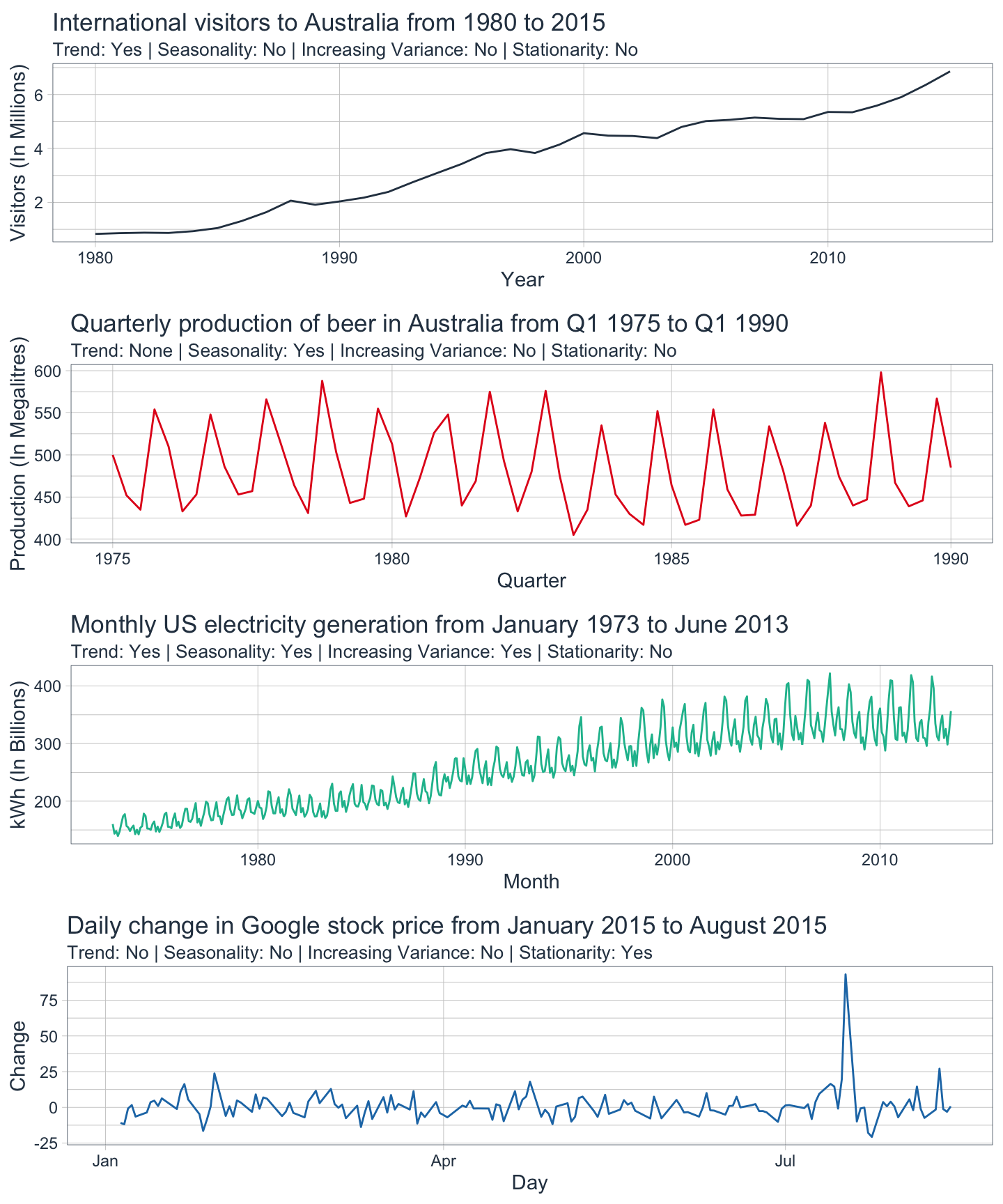
As a general rule, a time series without any long-term patterns is considered stationary.
1.5 Differencing
If a time series is not stationary, then an ARIMA model will not work properly. Therefore, the series must be made stationary by differencing the data. This process involves essentially subtracting observation 1 from observation 2, subtracting observation 2 from 3 and so on until an entirely new series of data is created.
- If a time series is non-stationary, then make it stationary through differencing.
- If a non-stationary time series is differenced, then the trend and seasonality is eliminated.
- If a time series is stationary, then the autocorrelation of the lags will drop to zero quickly.
- If a time series is non-stationary, then the autocorrelation of the lags will drop to zero slowly.
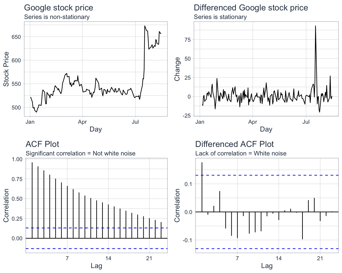
Notice how the ACF plot of the differenced stock price data has only one autocorrelation spike as opposed to the ACF plot of the original data which shows significant autocorrelation. This indicates that the differenced Google stock price data is stationary and looks just like random white noise i.e. the daily change is not correlated with past days. Differencing can be applied as many times as necessary to achieve stationarity.
1.6 What does ARIMA stand for?
The acronym ARIMA actually describes exactly which components are included in the model. They are as follows:
| Acronym | Component | Definition |
|---|---|---|
| AR | AutoRegression | AR models use multiple regression with lagged observations as predictors. They calculate a forecast by regressing on an observation and its lagged (i.e. prior) values. |
| I | Integrated | If included, this means that the actual values of the data have been replaced with the differences between each value and its prior value. This differencing is done to make the time series stationary. |
| MA | Moving Average | MA models use multiple regression with lagged errors as predictors. They calculate a forecast by regressing on the past forecast errors instead of the actual past values. |
1.7 What are the parameters in ARIMA models?
ARIMA models explicitly specify the above components as parameters. The standard notation of ARIMA(p,d,q) is used where the parameters (p,d,q) are given integer values to identify which kind of model it is.
| Parameter | Component | Definition |
|---|---|---|
| p | AutoRegression | The number of lags to include in the model a.k.a the lag order. |
| d | Integrated | The number of times the data has been differenced to make it stationary a.k.a the degree of differencing. |
| q | Moving Average | The number of past errors to include in the model i.e. the size of the moving average window a.k.a the order of moving average. |
For example, a notation of ARIMA(2,1,2) would indicate that the data has been differenced once (d) with 2 past observations (p) and 2 past errors (q) being included in the model.
One important thing to consider is that if a time series needs to be differenced d times to make it stationary, then the resulting model would be an ARIMA model. However, if a time series does not require any differencing because it is already stationary, then the resulting model would simply be an ARMA model. Essentially, an ARMA(p,q) model is equivalent to an ARIMA(p,0,q) model.
If your time series data has a seasonal pattern, then additional seasonal components (P,D,Q)m are added to the model. The seasonal components are similar to the non-seasonal components but they are backshifts of the seasonal period. For example, if you wanted to forecast sales for some product in February, you might predict that based on last February’s sales.
| Parameter | Component | Definition |
|---|---|---|
| P | Seasonal AutoRegression | The number of seasonal lags to include in the model a.k.a the seasonal lag order. |
| D | Integrated | The number of times the data has been seasonally-differenced to make it stationary a.k.a the seasonal differenced order. |
| Q | Seasonal Moving Average | The number of past seasonal errors to include in the model i.e. the size of the moving average window a.k.a the seasonal moving average order. |
| m | Time Steps | The number of time steps for a single seasonal period. |
It is best practice to apply only one order of seasonal differencing and up to two first differences to make data stationary. Click here to learn more about seasonal ARIMA models.
2. Transformations for Variance Stabilization
There are multiple ways to change time series data so that it becomes stationary. Some data show increasing variation as the level increases or just have unstable variance overall. In these cases, transforming the data to reduce the variance can be helpful.
- Transformations make fluctuations approximately even across the whole series.
- Simple transformations include square root, cube root, log, and inverse increasing in strength in this order.
- Box-Cox transformations do the same thing but are more complex mathematically.
The following examples will utilize a dataset containing the total monthly generation of electricity in kWh from 1973-2013 in the United States to show how to apply a transformation.
2.1 fpp2 Method: Box-Cox Transformation
# Plot original data
e1 <- autoplot(usmelec)

# Get best lambda value to make seasonal fluctuations about the same
lambda <- BoxCox.lambda(usmelec, method = "guerrero")

# Plot Box-Cox transformed data
e2 <- autoplot(BoxCox(usmelec,lambda))

# Arrange plots
plot_grid(e1, e2, nrow=2)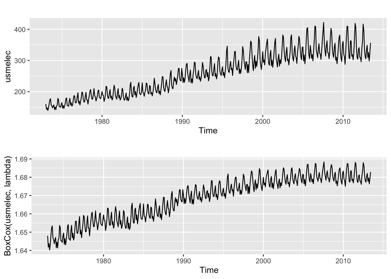
Note that the size of the seasonal fluctuations increases as the level increases in the original time series plot.
2.2 fpp3 Method: Box-Cox Transformation
# Convert ts to tsibble
elec_tsbl <- fpp2::usmelec %>%
  as_tsibble()

# Plot original data
e1 <- elec_tsbl %>%
  autoplot(value) +
  labs(title="US monthly net electricity generation")

# Get best lambda value to make seasonal fluctuations about the same
lambda <- elec_tsbl %>%
  features(value, features=guerrero) %>%
  pull(lambda_guerrero)

# Apply Box-Cox transformation to data using chosen lambda
elec_bc <- elec_tsbl %>%
  mutate(box_cox = box_cox(value, lambda))

# Plot data with Box-Cox transformation applied
e2 <- elec_bc %>%
  autoplot(box_cox) +
  labs(title="US monthly net electricity generation with Box-Cox transformation")

# Arrange plots
plot_grid(e1, e2, nrow=2)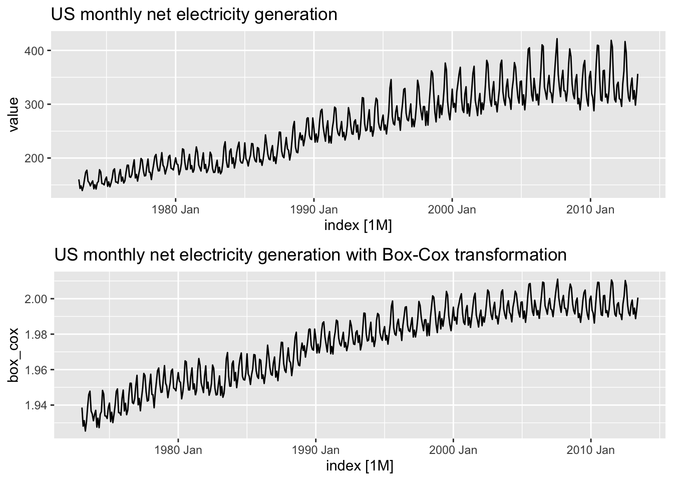
Note how the Box-Cox transformation stabilizes the variance as the level increases in the transformed plot.
2.3 modeltime Method: Box-Cox Transformation
Note: The modeltime framework can apply transformations during the model creation process as opposed to fpp2 and fpp3 where it is a separate process done beforehand. However, in this example the data will be transformed prior to model creation for illustrative purposes.
# Convert ts to tibble
elec_tbl <- fpp2::usmelec %>%
    tk_tbl(rename_index = "month") %>%
    mutate(month = as_date(month))

# Plot original data
e1 <- elec_tbl %>%
  plot_time_series(
      .date_var = month,
      .value    = value,
      .interactive = FALSE,
      .smooth_alpha = 0.4,
      .title = "US monthly net electricity generation"
  )

# Get best lambda value to make seasonal fluctuations about the same
lambda <- elec_tbl %>%
    as_tsibble() %>%   # Use fabletools as a workaround
    features(value, features=guerrero) %>%
    pull(lambda_guerrero)

# Apply Box-Cox transformation to data using chosen lambda
elec_bc_tbl <- elec_tbl %>%
  mutate(box_cox = box_cox(value, lambda))

# Plot data with Box-Cox transformation applied
e2 <- elec_bc_tbl %>%
    plot_time_series(
        .date_var = month,
        .value = box_cox,
        .interactive = FALSE,
        .smooth_alpha = 0.4,
        .title = "US monthly net electricity generation with Box-Cox transformation"
    )

# Arrange plots
plot_grid(e1, e2, nrow=2)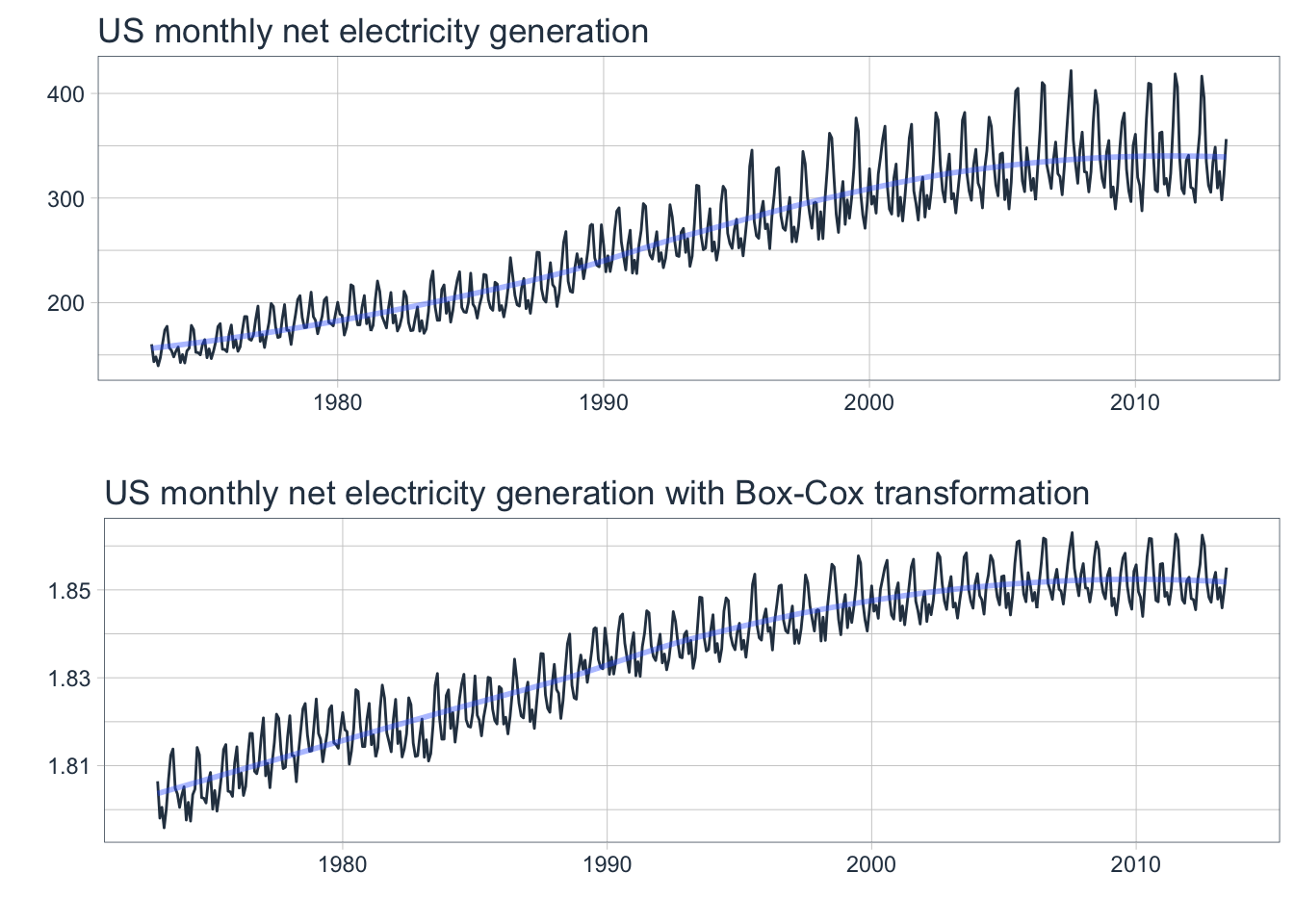
3. Non-seasonal differencing for stationarity
As noted earlier, ARIMA models require the data to be stationary. If a time series is not stationary, then it’s possible to apply a method called differencing to make it so. If this time series is also non-seasonal, then use lag-1 differences to model changes in observations.
3.1 fpp2 Method: Non-seasonal differencing
The following examples will use a dataset containing the annual female murder rate per 100,000 people in the United States from 1950-2004.
# Plot female murder rate
m1 <- autoplot(fpp2::wmurders) +
    labs(title="Female murder rate")

# Plot the differenced murder rate
m2 <- autoplot(diff(wmurders)) +
    ggtitle("Female murder rate (differenced)")

# Plot ACF of murder rate
m3 <- ggAcf(wmurders)

# Plot the ACF of the differenced murder rate
m4 <- ggAcf(diff(wmurders))

# Arrange plots
plot_grid(m1, m2, m3, m4, ncol=2)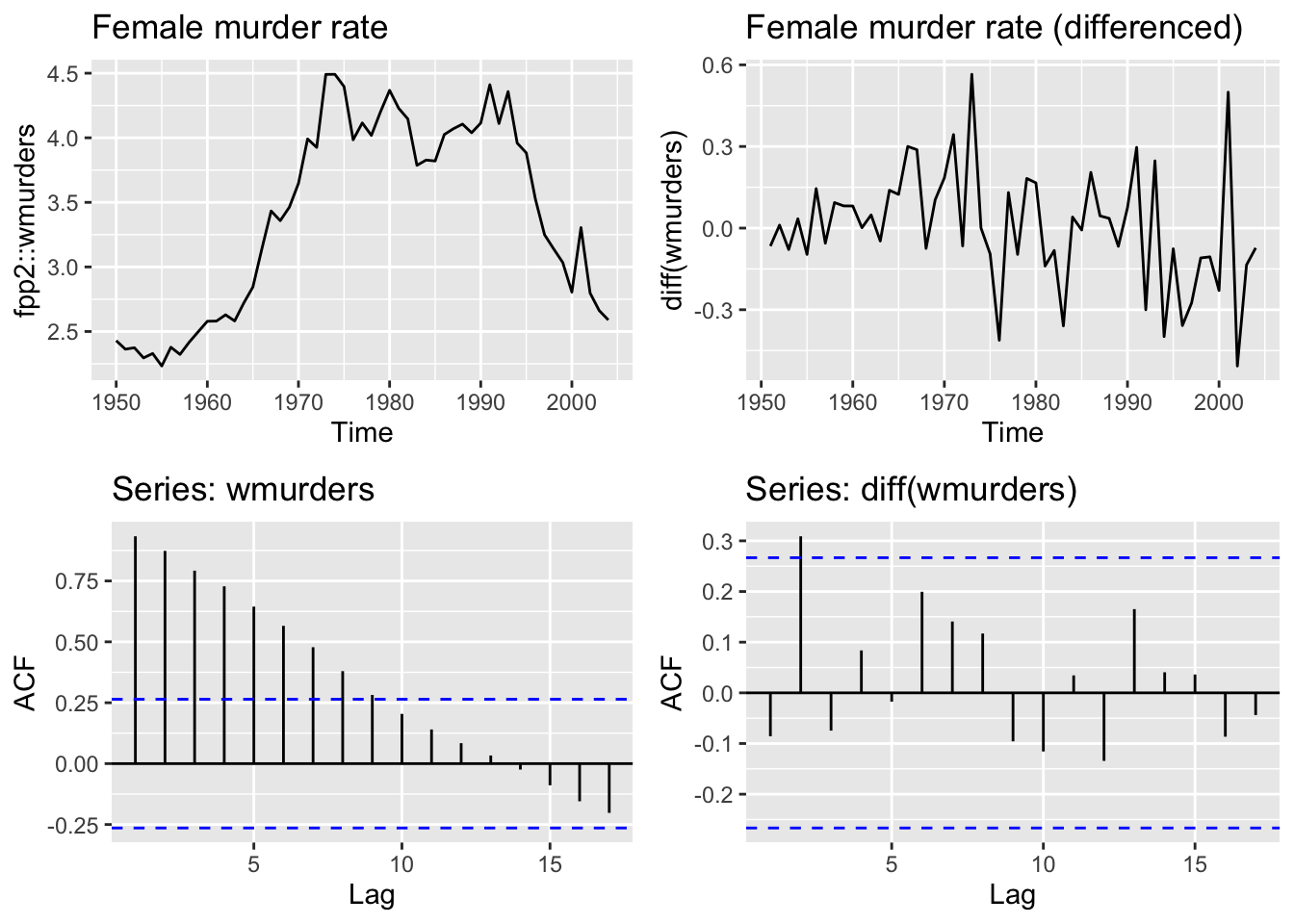
Does the differenced data look stationary?
3.2 fpp3 Method: Non-seasonal differencing
# Convert ts to tsibble
wmurders_tsbl <- fpp2::wmurders %>%
  as_tsibble() %>%
  mutate(diff_value = difference(value)) # Add differencing column

# Plot female murder rate
m1 <- wmurders_tsbl %>%
  autoplot(value) +
  labs(title="Female murder rate",
       x="", y="Per 100,000")

# Plot differenced murder rate
m2 <- wmurders_tsbl %>%
  autoplot(diff_value) +
  labs(title="Female murder rate (differenced)",
       x="", y="Difference")

# Plot ACF of murder rate
m3 <- wmurders_tsbl %>%
  ACF(value) %>%
  autoplot() +
  labs(title="ACF of murder rate",
       x="", y="ACF")

# Plot ACF of differenced murder rate
m4 <- wmurders_tsbl %>%
  ACF(diff_value) %>%
  autoplot() +
  labs(title="ACF of differenced murder rate",
       x="", y="ACF")

# Arrange plots
plot_grid(m1, m2, m3, m4, ncol=2)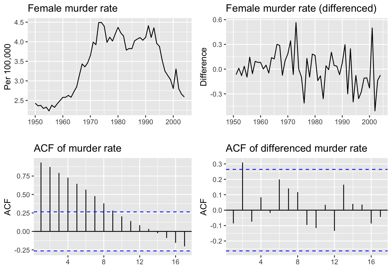
Does the ACF plot of the differenced data show significant autocorrelation left?
3.3 modeltime Method: Non-seasonal differencing
Note: The modeltime framework can apply transformations during the model creation process as opposed to fpp2 and fpp3 where it is a separate process done beforehand. However, in this example the data will be transformed prior to model creation for illustrative purposes.
# Convert ts to tibble
wmurders_tbl <- fpp2::wmurders %>%
    tk_tbl(rename_index = "year") %>%
    mutate(
        year = ymd(year, truncated = 2L),
        diff_value = difference(value)
        )

# Plot female murder rate
m1 <- wmurders_tbl %>%
    plot_time_series(
        .date_var = year,
        .value = value,
        .interactive = FALSE,
        .smooth_alpha = 0.4,
        .title = "Female murder rate"
    )

# Plot differenced murder rate
m2 <- wmurders_tbl %>%
    plot_time_series(
        .date_var = year,
        .value = diff_value,
        .interactive = FALSE,
        .smooth_alpha = 0.4,
        .title = "Differenced female murder rate"
    )

# Plot ACF/PACF of female murder rate
m3 <- wmurders_tbl %>%
    plot_acf_diagnostics(
        .date_var = year,
        .value = value,
        .lags = 20,
        .show_white_noise_bars = TRUE,
        .interactive = FALSE,
        .title="Lag diagnostics"
    )

# Plot ACF of differenced female murder rate
m4 <- wmurders_tbl %>%
    plot_acf_diagnostics(
        .date_var = year,
        .value = diff_value,
        .lags = 20,
        .show_white_noise_bars = TRUE,
        .interactive = FALSE,
        .title="Differenced lag diagnostics"
    )

# Arrange plots
plot_grid(m1, m2, m3, m4, ncol=2, rel_heights = c(1, 1.5))
The differenced data shows clear stationarity. The ACF & PACF plots of the differenced data shows very little autocorrelation as well with almost all lags within the white noise significance boundaries.
4. Seasonal differencing for stationarity
A first difference is the change between an observation and the next observation. A seasonal difference is the change between an observation and the previous observation from the prior season.
If a time series is non-seasonal but is also non-stationary, then you would apply first differencing as many times as necessary to make it stationary.
If a time series is seasonal and thus by definition non-stationary, then apply a seasonal difference to try and make it stationary. If this seasonally differenced series is still non-stationary, then apply first differencing until it is stationary.
The following examples will utilize a dataset containing the monthly corticosteroid expenditure in millions of dollars in Australia from 1991-2008 to illustrate the seasonal differencing process.
This non-stationary time series would benefit from applying a transformation before differencing. Since the variance is not greatly increasing with the level, it probably does not require a Box-Cox transformation. Instead, let’s try a log transformation.
4.1 fpp2 Method: Seasonal Differencing
# Filter & summarize then convert tsibble to ts
h02_ts <- tsibbledata::PBS %>%
    filter(ATC2 == "H02") %>%
    summarise(Cost = sum(Cost) / 1e6) %>%
    as.ts()

# Plot monthly corticosteroid drug expenditure in millions
h1 <- autoplot(h02_ts)

# Transform data with log & seasonal differencing
diff_log_h02_ts <- diff(log(h02_ts), lag = 12)  # Monthly = 12 periods

# Plot logged & seasonally-differenced monthly expenditure
h2 <- autoplot(diff_log_h02_ts)

# Arrange plots
plot_grid(h1, h2, nrow=2)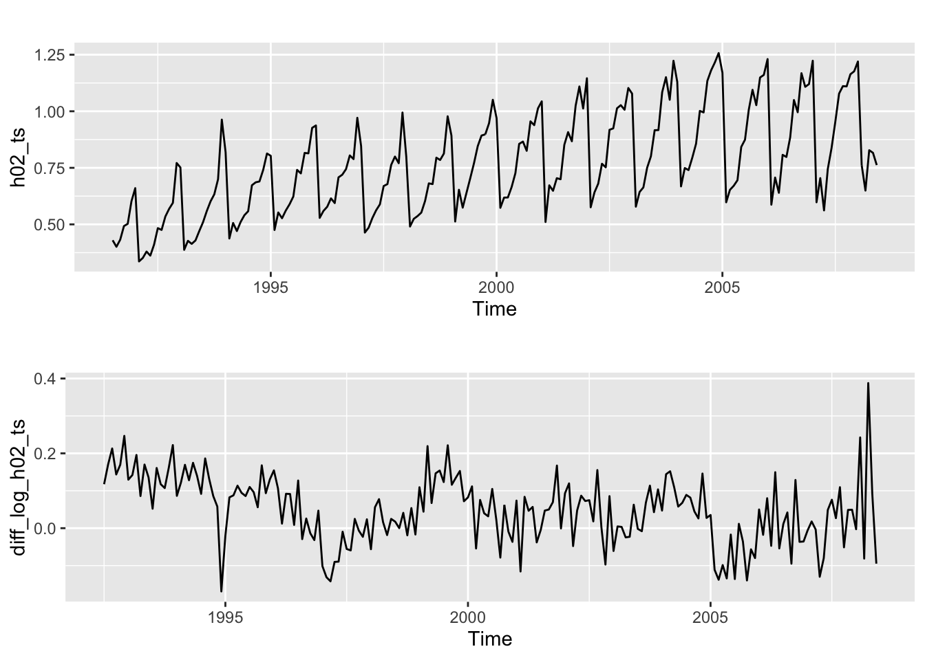
Although the data has been transformed logarithmically and seasonally-differenced once, it is still non-stationary as there is some noticeable trend. Try differencing the data again.
# Transform still non-stationary data with another degree of differencing
dbl_diff_log_h02_ts <- diff(diff_log_h02_ts)

# Plot logged & doubly differenced monthly expenditure
h3 <- autoplot(dbl_diff_log_h02_ts)

# Plot ACF of doubly-differenced monthly expenditure
h4 <- ggAcf(dbl_diff_log_h02_ts)

# Arrange plots
plot_grid(h3, h4, ncol=1)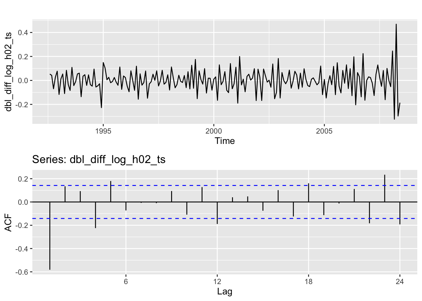
Although the data is now stationary, there are still some significant autocorrelation spikes. However, this is the expected behavior with seasonal data.
4.2 fpp3 Method: Seasonal Differencing
# Transform logarithmically, apply seasonal + first differencing, plot it
h02_tsbl_long <- PBS %>%
  filter(ATC2 == "H02") %>%
  summarise(Cost = sum(Cost) / 1e6) %>%
  transmute(
      `Sales ($million)` = Cost,
      `Log sales` = log(Cost),  # Transform using log
      `Annual change in log sales` = difference(log(Cost), 12), # Calculate seasonal differences
      `Double differenced log sales` = difference(difference(log(Cost), 12), 1)) %>%
  gather("Type", "Sales", !!!syms(measured_vars(.)), factor_key=TRUE)

# Facet plot by Type
h02_tsbl_long %>%
  ggplot(aes(x=Month, y=Sales)) +
  geom_line() +
  facet_grid(vars(Type), scales="free_y") +
  labs(title = "Corticosteroid drug sales", x = "Year", y = "")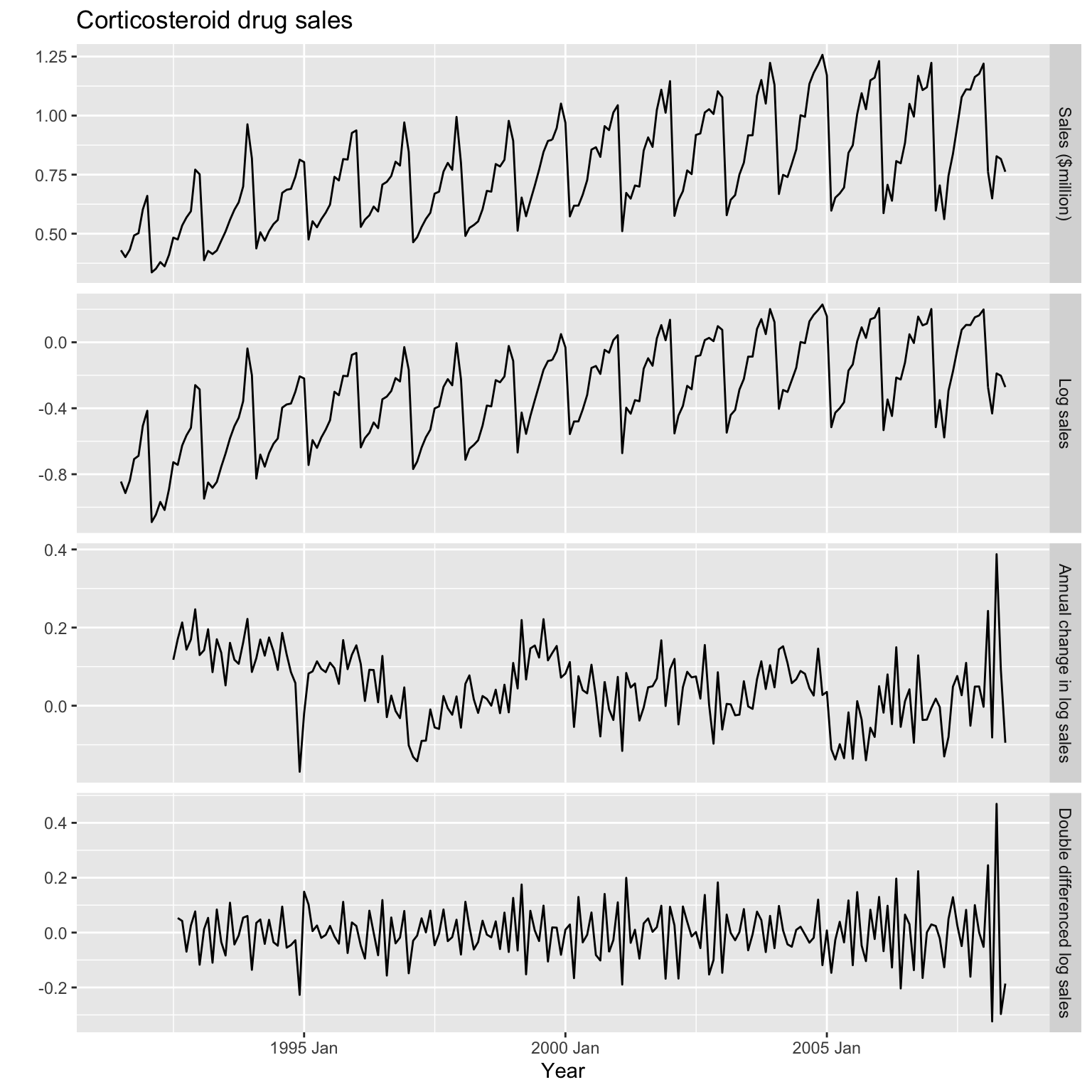
4.3 modeltime Method: Seasonal Differencing
# Convert tsibble to tibble
h02_tbl_long <- h02_tsbl_long %>%
  tk_tbl(preserve_index = FALSE) %>%
  mutate(Month = as_date(Month))

# Facet plot by Type
h02_tbl_long %>%
  plot_time_series(
      .date_var = Month,
      .value = Sales,
      .facet_vars = Type,
      .smooth_alpha = 0.6,
      .interactive = FALSE,
      .title = "Corticosteroid drug sales")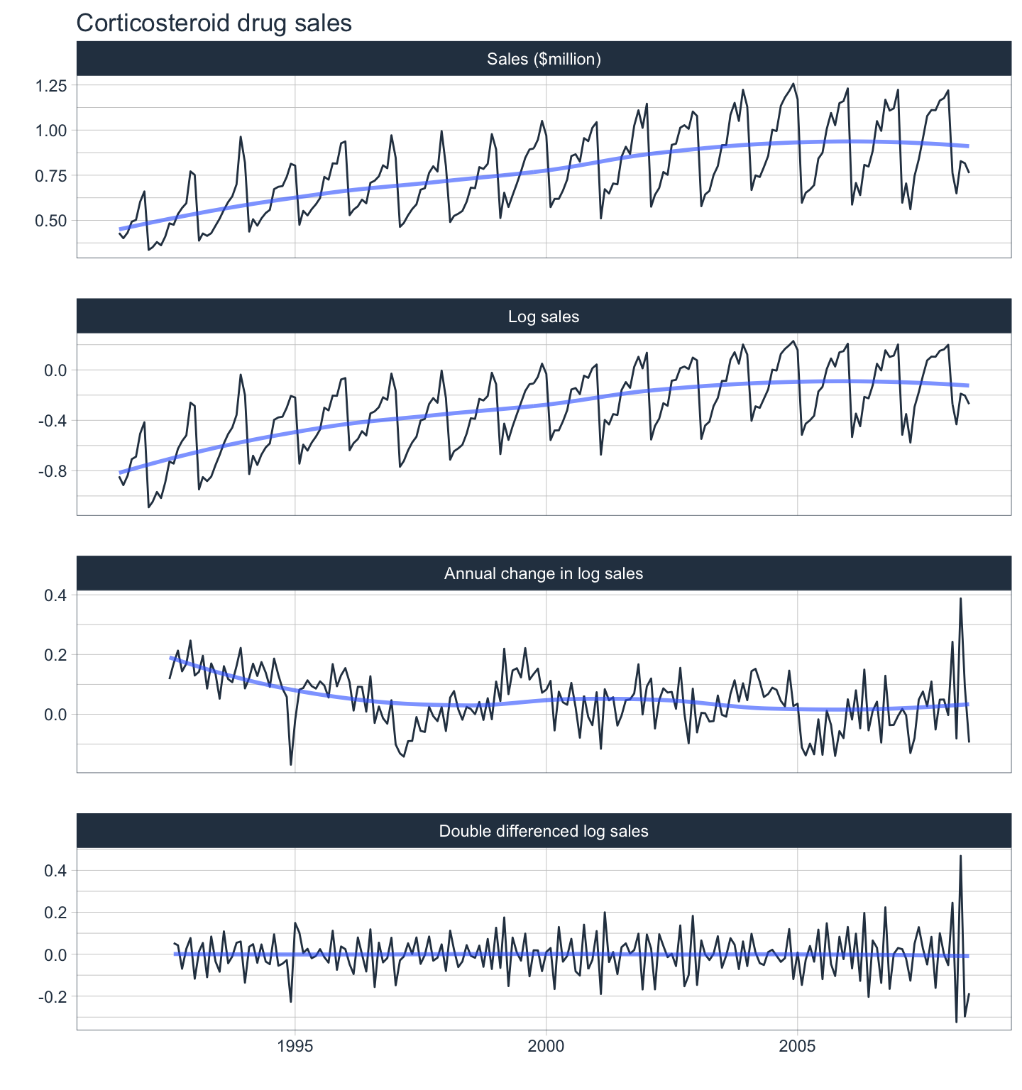
One handy feature of
modeltimeandtimetkis the use of a LOESS smoother which can help in determining the stationarity of a series.
5. The ARIMA Modeling Process
There are two methods for fitting ARIMA models to time series data. One method is a manual process which involves analyzing the ACF and PACF plots to select a model based on what is found. The other method is to use the Hyndman-Khandakar algorithm to automatically choose an ARIMA model. It’s important to know that automatically choosing a model does not guarantee the best fitting model as we will see down below.
5.1 Manual ARIMA Modeling
The way to choose an ARIMA model manually can be a quite involved process. The following is derived from Professor Hyndman’s excellent book which describes a general procedure for manually choosing an ARIMA model for non-seasonal data.
| Step | Process |
|---|---|
|
|
Plot the data and identify any unusual observations. |
|
|
If the variance is unstable, then apply a transformation (log, Box-Cox, etc.) to stabilize it. |
|
|
If the data are not stationary, then take first differences until the data are stationary. |
|
|
Plot ACF and PACF and identify whether ARIMA(p,d,0) or ARIMA(0,d,q) is more appropriate. |
|
|
Manually fit multiple models and find the lowest AICc. |
|
|
Plot ACF of the residuals and do a portmanteau test to make sure they look like white noise. If not, go back to step 5. |
|
|
Once the residuals look like white noise, calculate forecasts. |
5.2 Automatic ARIMA Modeling
All three forecasting frameworks rely on the Hyndman-Khandakar algorithm to automatically choose an ARIMA model. The algorithm uses a combination of unit root tests, minimization of the AICc score, as well as maximum likelihood estimation to automatically choose the best model.
It is important to know that it also uses approximations and a stepwise approach to speed up the search for a model by default. It’s possible to search a much larger set of ARIMA models if you do not use either methods but it will take longer. Here’s a general procedure for automatically choosing an ARIMA model for non-seasonal data:
| Step | Process |
|---|---|
|
|
Plot the data and identify any unusual observations. |
|
|
If the variance is unstable, then apply a transformation (log, Box-Cox, etc.) to stabilize it. |
|
|
Automatically fit multiple models and find the lowest AICc. |
|
|
Plot ACF of the residuals and do a portmanteau test to make sure they look like white noise. |
|
|
Once the residuals look like white noise, calculate forecasts. |
Although automatically choosing a model can speed things up, manually testing the residuals for white noise is still recommended before calculating forecasts.
6. Automatic ARIMA Modeling for Non-Seasonal Time Series
The following example will utilize a dataset containing the growth rates of personal consumption and personal income in the United States.
6.1 fpp2 Method: Auto-ARIMA | Non-Seasonal
# 1. Plot the data and identify any unusual observations.
autoplot(fpp2::austa) +
    labs(title = "International visitors to Australia from 1980-2015",
        x = "Year", y="Millions")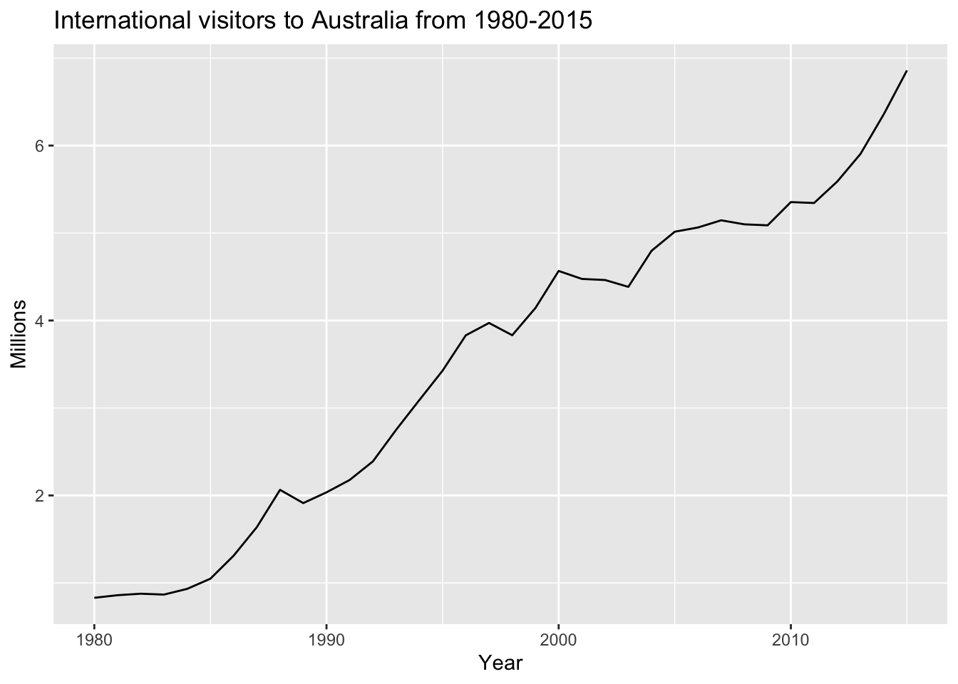
Since there is no seasonal pattern in this series, apply a non-seasonal ARIMA model. Since the variance is stable, there is no need to transform this series and we can skip step 2.
# 3. Automatically fit multiple models and find the lowest AICc.
fit_austa_ts <- auto.arima(austa, seasonal = FALSE)

# Check the model report
summary(fit_austa_ts)
## Series: austa
## ARIMA(0,1,1) with drift
##
## Coefficients:
## ma1 drift
## 0.3006 0.1735
## s.e. 0.1647 0.0390
##
## sigma^2 estimated as 0.03376: log likelihood=10.62
## AIC=-15.24 AICc=-14.46 BIC=-10.57
##
## Training set error measures:
## ME RMSE MAE MPE MAPE MASE
## Training set 0.0008313383 0.1759116 0.1520309 -1.069983 5.513269 0.7461559
## ACF1
## Training set -0.000571993# 4. Plot ACF of the residuals and do a portmanteau test to make sure they look like white noise.
checkresiduals(fit_austa_ts)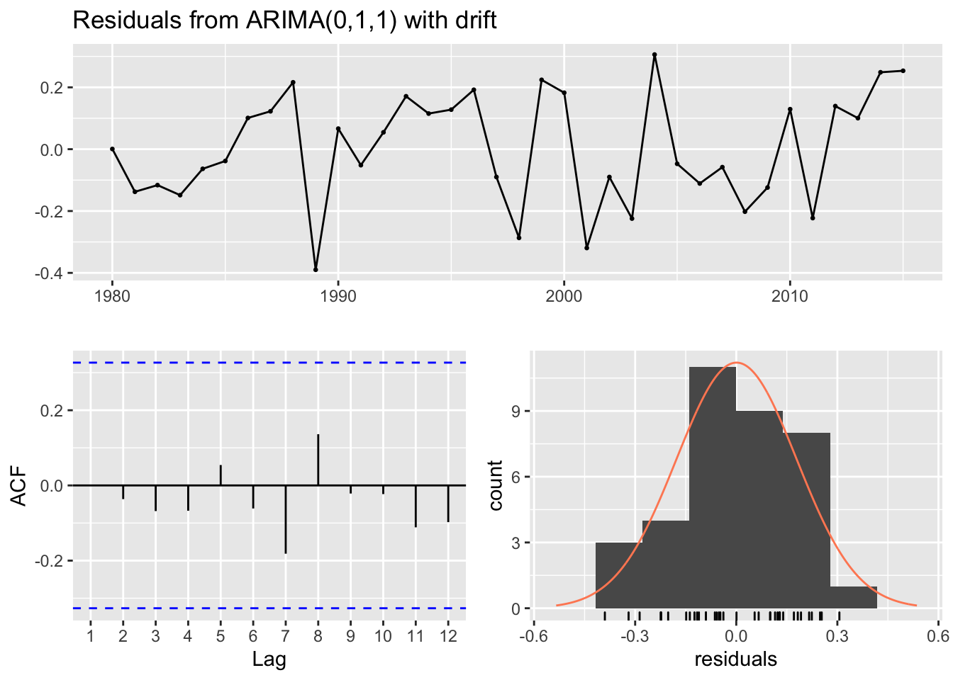
##
##  Ljung-Box test
##
## data:  Residuals from ARIMA(0,1,1) with drift
## Q* = 2.297, df = 5, p-value = 0.8067
##
## Model df: 2.   Total lags used: 7
The residuals plot shows a mean around 0, the ACF does not show any significant autocorrelation and the Ljung-Box test shows a p-value greater than 0.05. These factors confirm that the residuals can be considered to be white noise. The distribution is also mostly normal without outliers which means the prediction intervals will be less wide and that is a good thing.
# 5. Once the residuals look like white noise, calculate forecasts.
autoplot(forecast(fit_austa_ts, h=10)) +
    labs(x = "Year", y="Millions")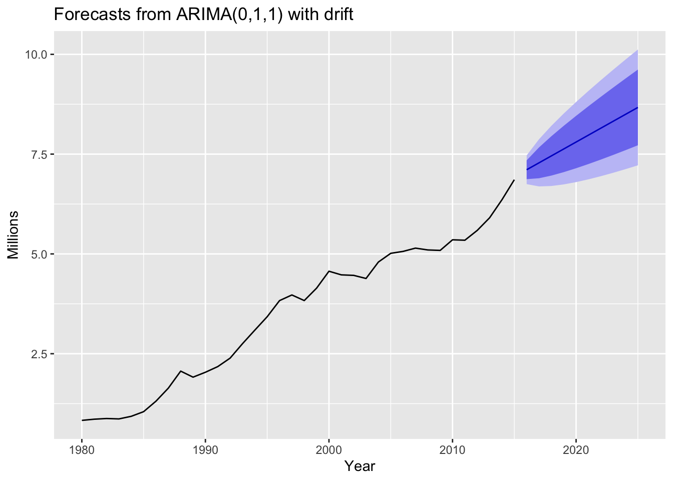
The automatically chosen ARIMA(0,1,1) with drift accounts for the trend seen in the data and produces reasonable forecasts with good prediction intervals.
6.2 fpp3 Method: Auto-ARIMA | Non-Seasonal
The following example will utilize a dataset containing the percentage of GDP for exports in Egypt from 1960-2017.
# 1. Plot the data and identify any unusual observations.
egypt_tsbl <- tsibbledata::global_economy %>%
  filter(Code == "EGY") %>%
  select(Year, Exports)

egypt_tsbl %>% gg_tsdisplay(Exports, plot_type = "partial")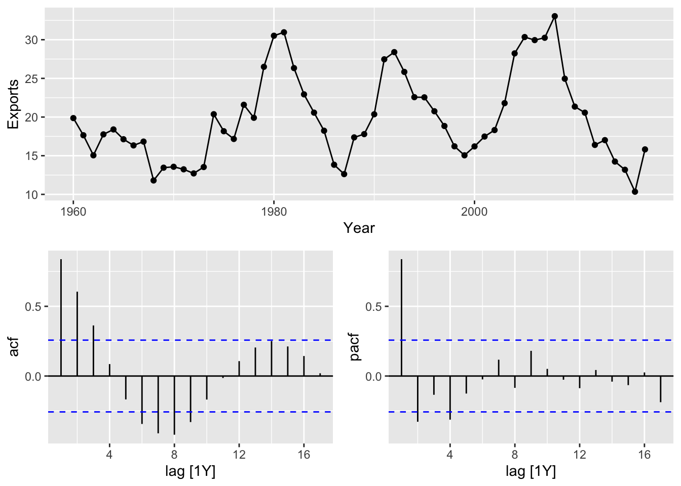
There is no seasonal pattern in this series and the variance is stable so there is no need for differencing. Since the series also shows cyclic behavior without trend or seasonality, it is considered stationary. When the data are seasonal or cyclic, the ACF plot will show peaks around the seasonal lags or at the average cycle length respectively i.e. ACF plots for seasonal and cyclic data may look similar which can be misleading. Since the data is stationary, we can skip step 2.
# 3. Automatically fit multiple models and find the lowest AICc.
fit_egypt_tsbl <- egypt_tsbl %>% model(ARIMA(Exports))

# Check the model report
report(fit_egypt_tsbl)
## Series: Exports
## Model: ARIMA(2,0,1) w/ mean
##
## Coefficients:
## ar1 ar2 ma1 constant
## 1.6764 -0.8034 -0.6896 2.5623
## s.e. 0.1111 0.0928 0.1492 0.1161
##
## sigma^2 estimated as 8.046: log likelihood=-141.57
## AIC=293.13 AICc=294.29 BIC=303.43# 4. Plot ACF of the residuals and do a portmanteau test to make sure they look like white noise.
fit_egypt_tsbl %>% gg_tsresiduals()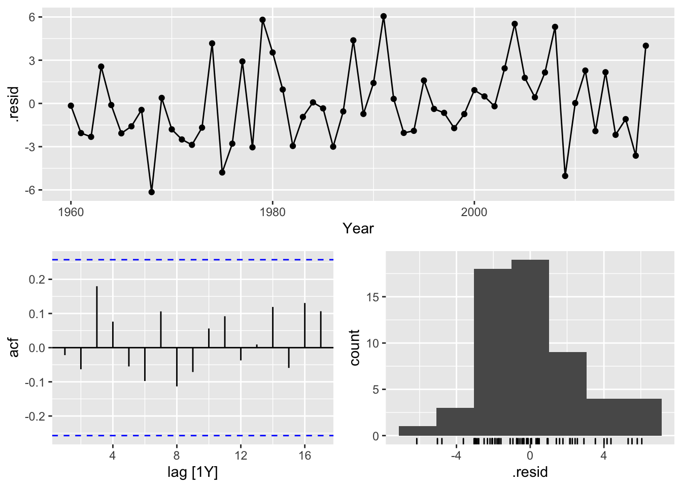
# Check if the residuals are white noise with a Ljung-Box test
fit_egypt_tsbl %>%
  augment() %>%
  select(Year, .resid) %>%
  features(.resid, ljung_box, lag=10)
## # A tibble: 1 x 2
## lb_stat lb_pvalue
## <dbl> <dbl>
## 1 5.78 0.833The residuals plot shows a mean around 0, the ACF does not show any significant autocorrelation and the Ljung-Box test shows a p-value greater than 0.05. These factors confirm that the residuals can be considered to be white noise. The distribution is skewed a bit left which means the prediction intervals will be wider which isn’t great but is acceptable.
# 5. Once the residuals look like white noise, calculate forecasts.
fit_egypt_tsbl %>%
  forecast(h = 10) %>%
  autoplot(egypt_tsbl) +
  labs(
    title = "Egyptian Exports of Goods and Services 10-year forecasts",
    subtitle = "ARIMA(2,0,1) w/ mean model",
    y = "% of GDP")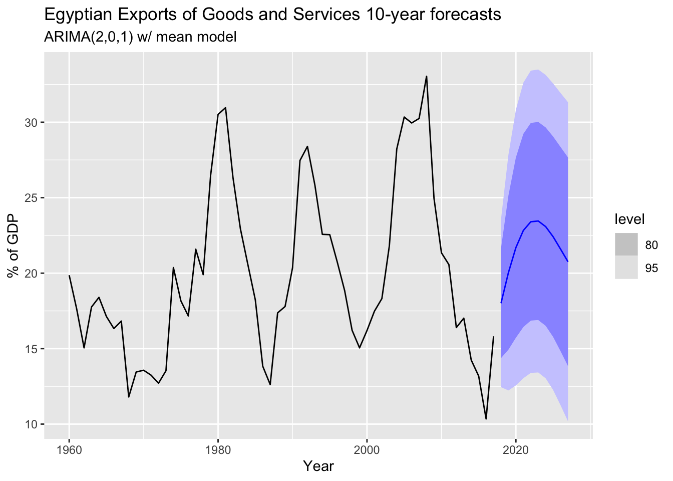
The automatically chosen ARIMA(2,0,1) w/ mean model accounts for the cyclic nature of the data.
6.3 modeltime Method: Auto-ARIMA | Non-Seasonal
The following example will utilize a dataset containing the quarterly percentage changes in economic consumption in the United States from 1970-2019.
# Convert tsibble to tibble
us_change_tbl <- fpp3::us_change %>%
  select(Quarter, Consumption) %>%
  tk_tbl(preserve_index = FALSE) %>%
  mutate(Quarter = as_date(Quarter))

# 1. Plot the data and identify any unusual observations.
us_change_tbl %>%
  plot_time_series(
    .date_var = Quarter,
    .value = Consumption,
    .smooth_alpha = 0.6,
    .interactive = FALSE,
    .title = "Quarterly percent changes in US consumption expenditure"
  )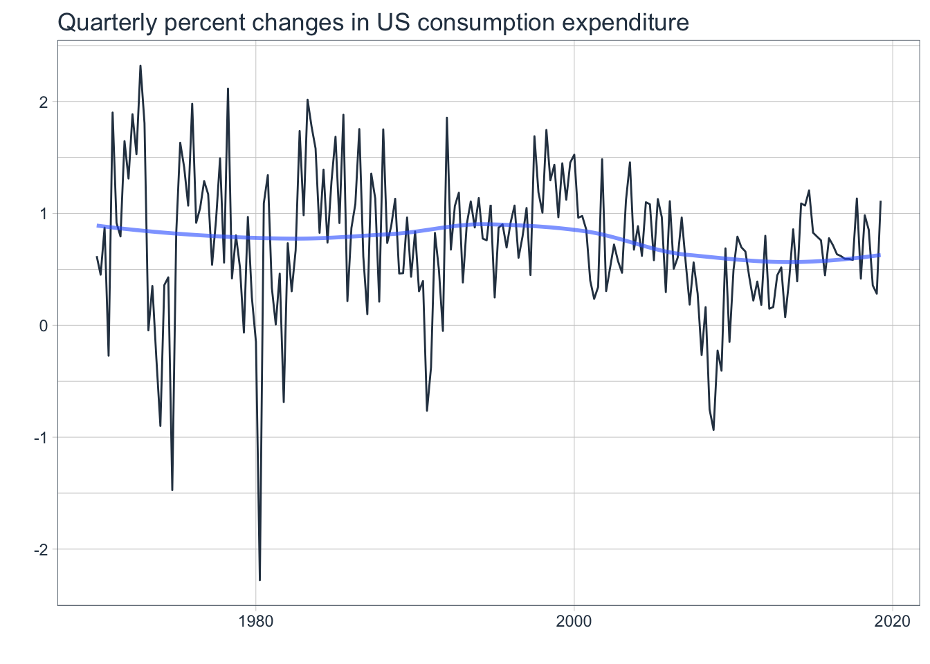
This is a quarterly series but there is no obvious seasonal pattern. There is also no trend and the variance does not seem to change much. It does not need differencing as it is already stationary and would be a good candidate for fitting a non-seasonal ARIMA model.
# 3. Automatically fit multiple models and find the lowest AICc.

# Split the data 80/20
splits <- rsample::initial_time_split(us_change_tbl, prop = 0.8)

# Model Spec
model_spec_arima <- arima_reg() %>%
  set_engine("auto_arima")

# Fit Spec
model_fit_arima <- model_spec_arima %>%
  fit(Consumption ~ Quarter, data = rsample::training(splits))
## frequency = 4 observations per 1 year# Check model report
model_fit_arima## parsnip model object
##
## Fit time: 1.1s
## Series: outcome
## ARIMA(1,0,2)(2,0,2)[4] with non-zero mean
##
## Coefficients:
## ar1 ma1 ma2 sar1 sar2 sma1 sma2 mean
## 0.7942 -0.5871 0.1229 0.7715 -0.6596 -0.8596 0.5943 0.7608
## s.e. 0.0985 0.1207 0.1095 0.5075 0.5037 0.5048 0.5761 0.1052
##
## sigma^2 estimated as 0.4009: log likelihood=-148.22
## AIC=314.45 AICc=315.67 BIC=342.01# 4. Plot ACF of the residuals and do a portmanteau test to make sure they look like white noise. If not white noise, then search a larger set of models to choose from.
# Create table of model to use
auto_arima_model_tbl <- modeltime_table(model_fit_arima)
# Calibrate the model to produce confidence intervals
arima_calibration_tbl <- auto_arima_model_tbl %>%
modeltime_calibrate(new_data = rsample::testing(splits))
# Create residuals table
arima_residuals_tbl <- arima_calibration_tbl %>% modeltime_residuals()
# Plot the residuals
u1 <- arima_residuals_tbl %>%
plot_modeltime_residuals(
.type = "timeplot",
.interactive = FALSE)
u2 <- arima_residuals_tbl %>%
plot_modeltime_residuals(
.type = "acf",
.interactive = FALSE,
.title = "ACF and PACF Plots")
# Check for white noise with a Ljung-Box test
arima_residuals_tbl %>%
select(.residuals, .index) %>%
as_tsibble() %>% # fabletools workaround
features(.residuals, ljung_box, lag=24, dof=0)## # A tibble: 1 x 2
## lb_stat lb_pvalue
## <dbl> <dbl>
## 1 34.4 0.0779# Arrange plots
plot_grid(u1, u2, ncol=1)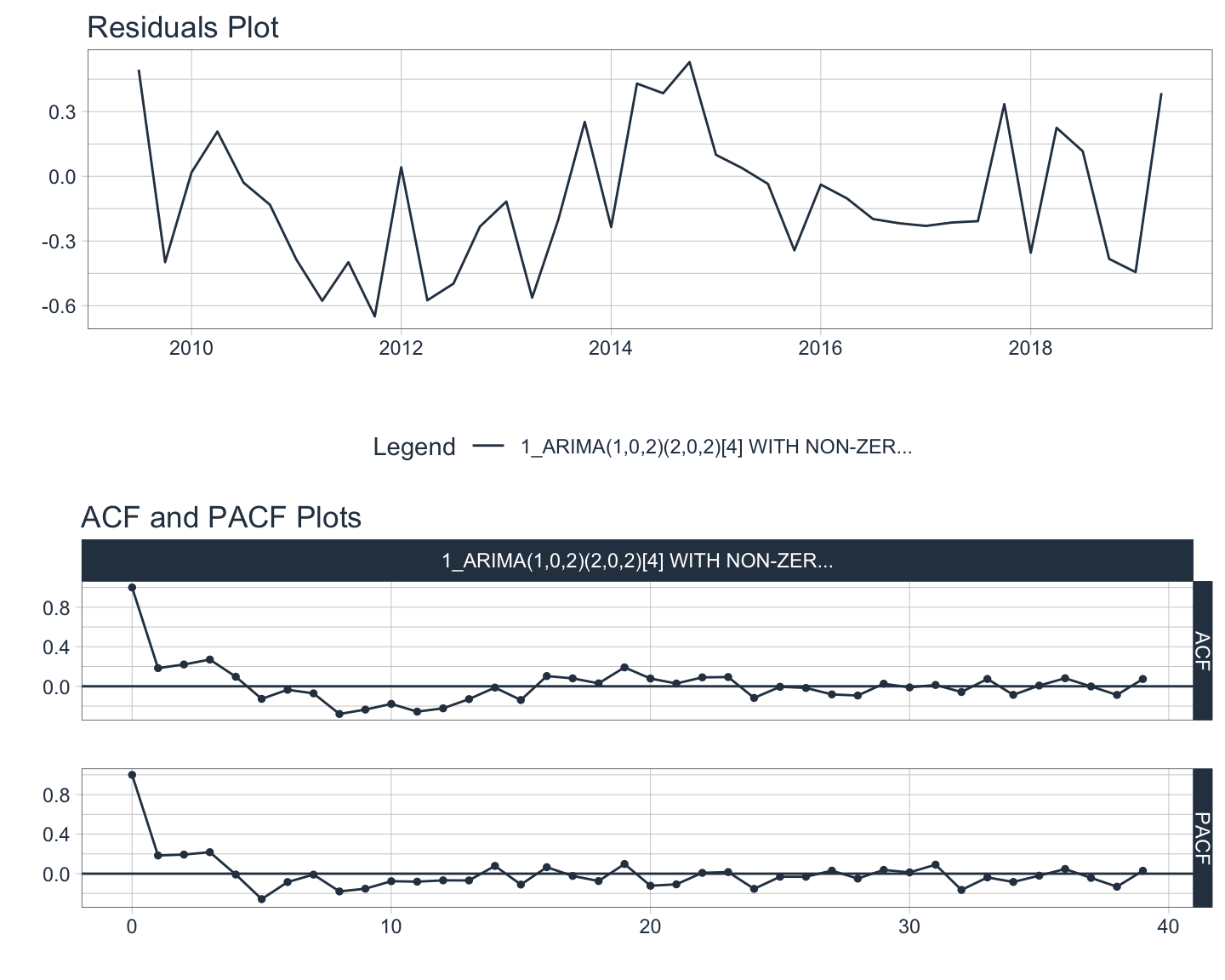
Although the ACF plot shows some autocorrelation remaining in the test set, the residuals pass the Ljung-Box test with a p-value of approximately 0.078 which is higher than the significance threshold of 0.05. It is important to know that not every model will pass all of the tests for white noise and that is okay. However, the automatically chosen ARIMA model here should forecast well. Of interest is that the algorithm chose a seasonal model for this seemingly non-seasonal data.
# 5. Once the residuals look like white noise, calculate forecasts.
arima_calibration_tbl %>%
  modeltime_forecast(
      new_data = rsample::testing(splits),
      actual_data = us_change_tbl,
      h = "5 years"
  ) %>%
  plot_modeltime_forecast(
      .legend_max_width = 25,
      .interactive = TRUE,
      .title = "Quarterly changes in US consumption expenditure 5-year forecasts",
      .x_lab = "Quarter",
      .y_lab = "Percent Change"
  ) %>%
  plotly::layout(  # Custom ggplotly layout
    legend = list(
      orientation = "h",   # Show model names horizontally
      xanchor = "center",  # Use center of legend as anchor
      x = 0.5, # Legend in center of x-axis
      y = -0.2) # Place legend below x-axis
    )
The ARIMA(1,0,2)(2,0,2)[4] with non-zero mean model accounts for the somewhat cyclic nature of the series and provides reasonable forecasts with decent confidence intervals.
7. Automatic ARIMA Modeling for Seasonal Time Series
The auto-ARIMA process for seasonal data is a bit more complex but mostly similar to the non-seasonal process.
7.1 fpp2 Method: Auto-ARIMA | Seasonal
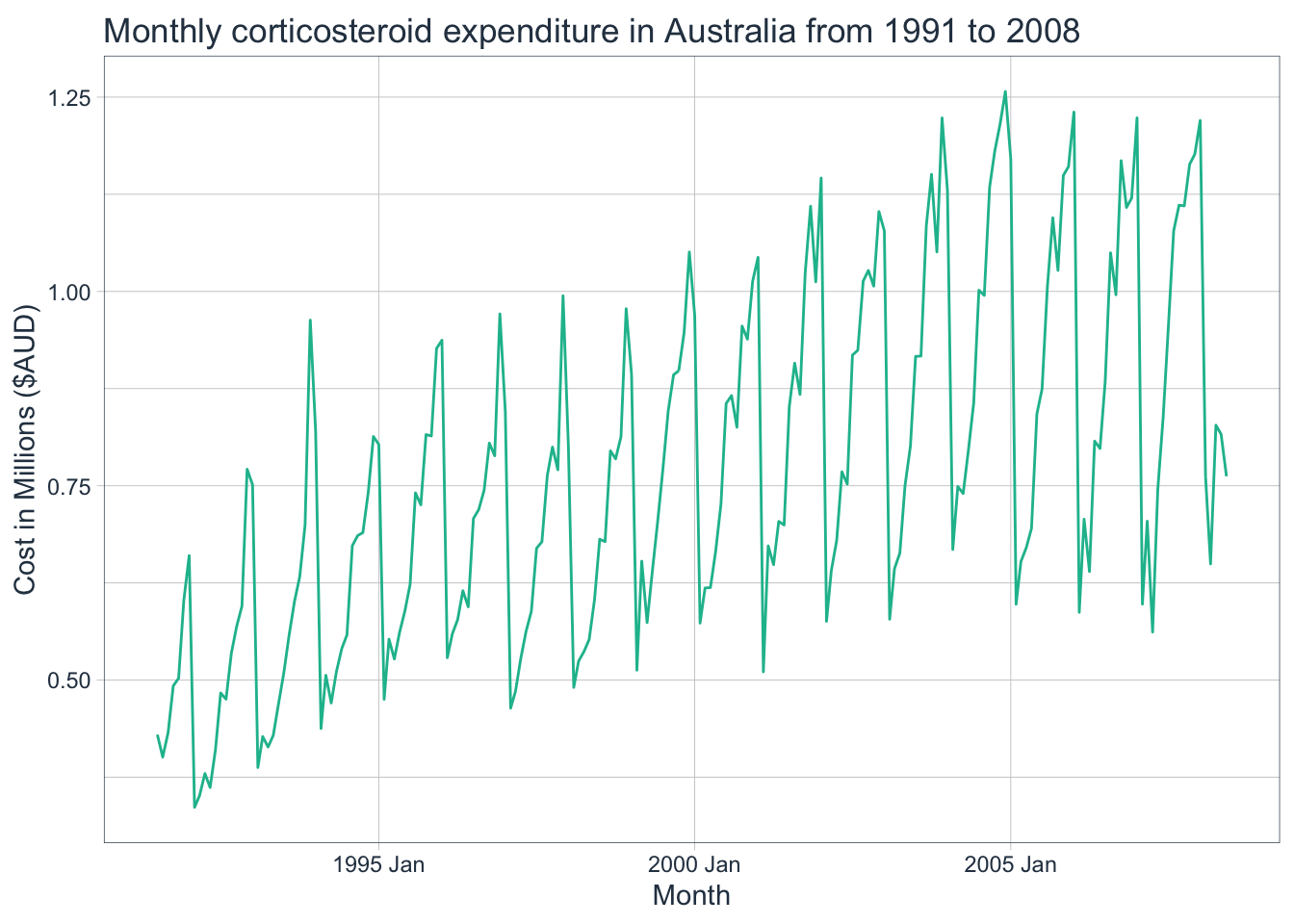
The following example will utilize a dataset containing the monthly corticosteroid expenditure in millions of dollars in Australia from 1991-2008. It is the same dataset used in section 4 above.
# 1.Plot the data and identify any unusual observations.
autoplot(h02_ts) +
  labs(title = "Monthly corticosteroid expenditure in Australia from 1991 to 2008",
         x = "Month", y = "Cost in Millions ($AUD)")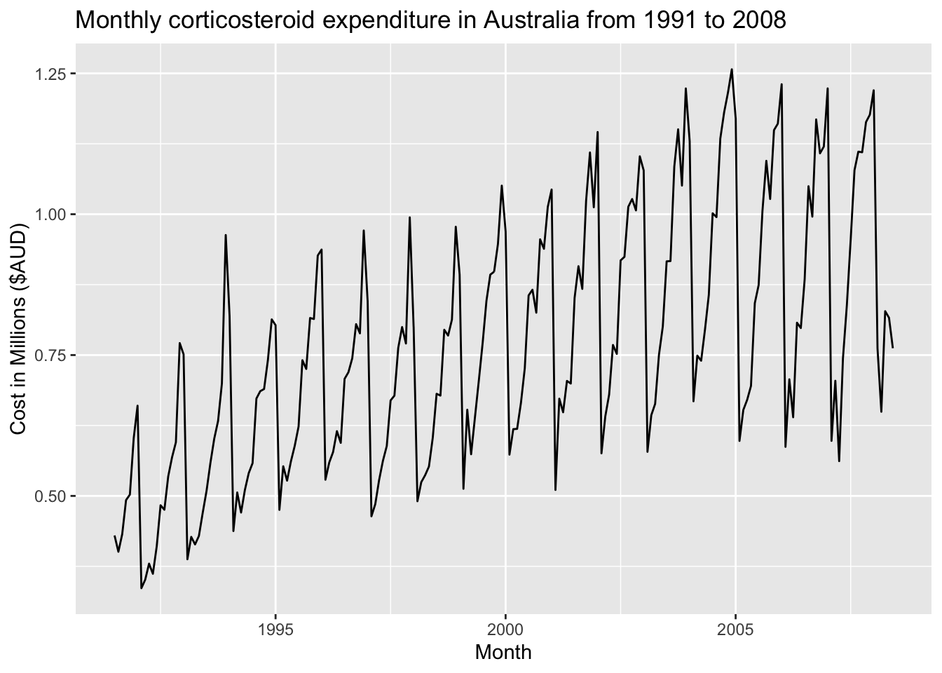
As noted earlier, this series has increasing variance as the level increases and would benefit from a transformation. It will also require seasonal differencing to make it stationary.
# 1. Plot the data and identify any unusual observations.
# 2. If the variance is unstable, then apply a transformation to stabilize it.

cbind("H02 sales (scripts in millions)" = h02_ts,
      "Log H02 sales" = log(h02_ts),
      "Seasonally differenced" = diff(log(h02_ts), lag = 12)) %>% # Yearly = 12 lags
  autoplot(facets=TRUE) +
  labs(title="Corticosteroid drug sales in Australia",
    x="Year",y="")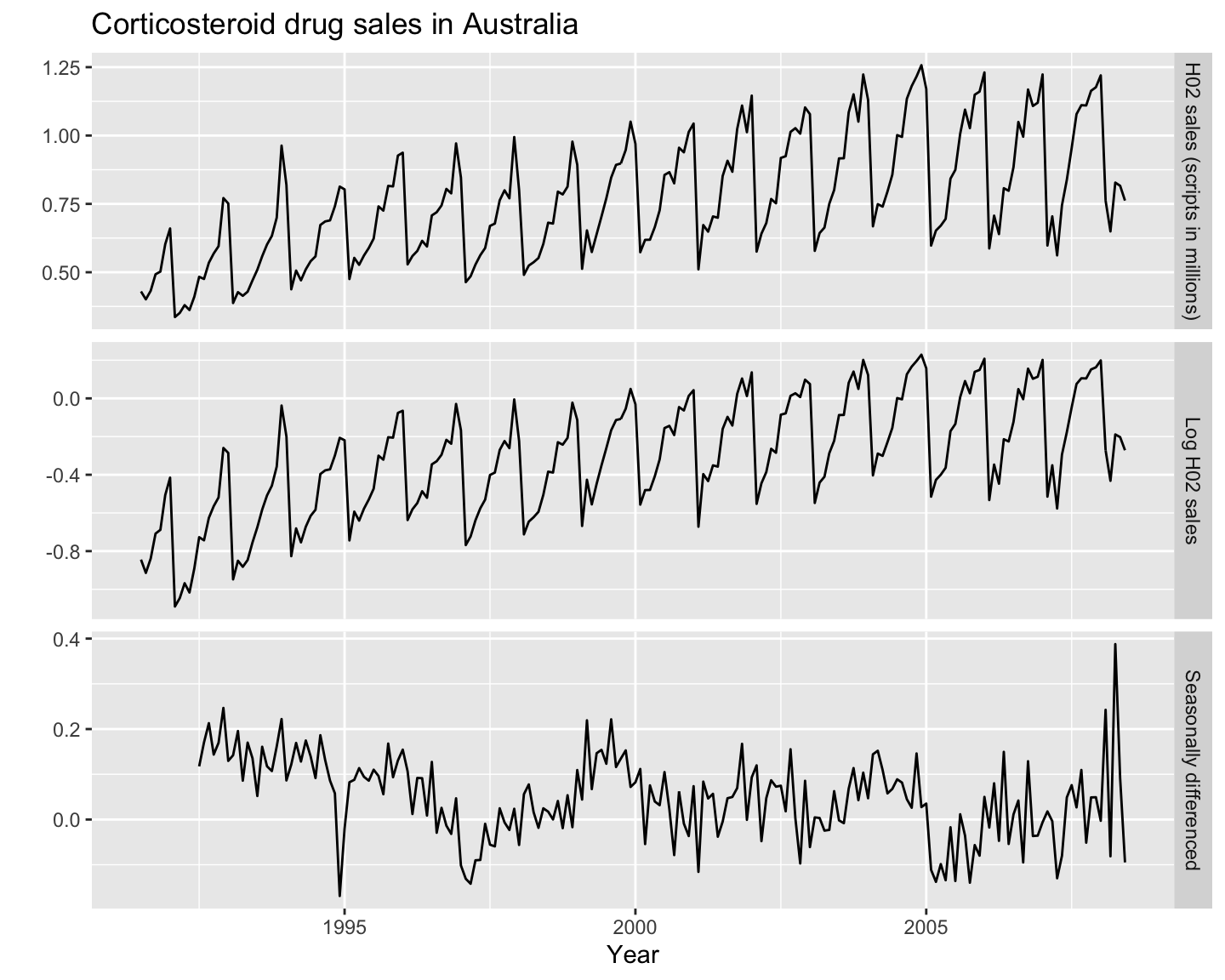
After applying a log transformation and seasonal differencing, the series is now stationary and is ready to automatically fit an ARIMA model.
# 3. Automatically fit multiple models and find the lowest AICc.
fit_h02_ts <- auto.arima(h02_ts, lambda = 0)

# Check model report
summary(fit_h02_ts)
## Series: h02_ts
## ARIMA(2,1,1)(0,1,2)[12]
## Box Cox transformation: lambda= 0
##
## Coefficients:
## ar1 ar2 ma1 sma1 sma2
## -1.1358 -0.5753 0.3683 -0.5318 -0.1817
## s.e. 0.1608 0.0965 0.1884 0.0838 0.0881
##
## sigma^2 estimated as 0.004278: log likelihood=248.25
## AIC=-484.51 AICc=-484.05 BIC=-465
##
## Training set error measures:
## ME RMSE MAE MPE MAPE MASE
## Training set -0.003931805 0.0501571 0.03629816 -0.5323365 4.611253 0.5987988
## ACF1
## Training set -0.003740267# 4. Plot ACF of the residuals and do a portmanteau test to make sure they look like white noise.
checkresiduals(fit_h02_ts, lag=36)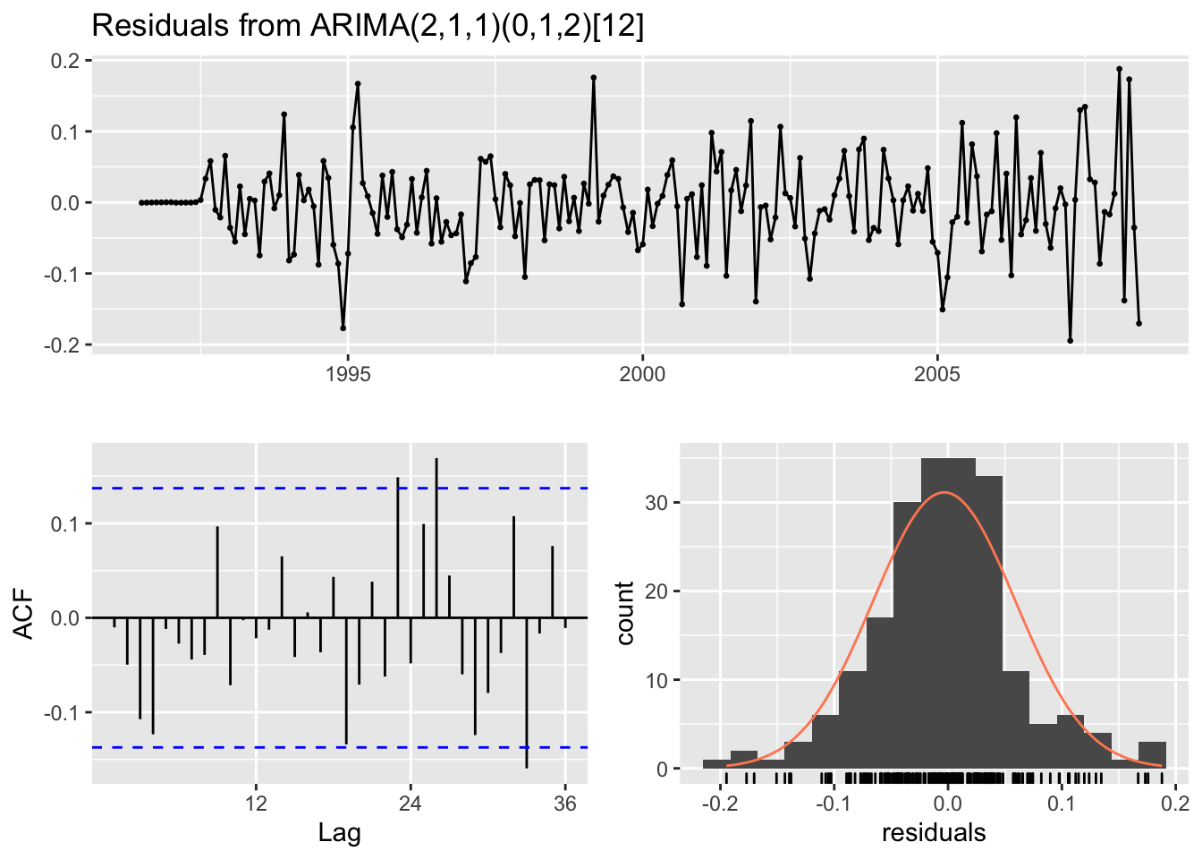
##
##  Ljung-Box test
##
## data:  Residuals from ARIMA(2,1,1)(0,1,2)[12]
## Q* = 51.096, df = 31, p-value = 0.01298
##
## Model df: 5.   Total lags used: 36
There is some autocorrelation shown in the ACF plot and the model fails the Ljung-Box test. The model can still be used for forecasting even though the residuals do not look like white noise (i.e. they are correlated); however, the prediction intervals will probably be inaccurate. Nothing is perfect; it is possible that none of your models will pass all of the residual tests for white noise but that does not mean they can’t be used for forecasting.
# 5. Once the residuals look like white noise, calculate forecasts.
fit_h02_ts %>%
  forecast(h = 24) %>% # 2-year forecasts
  autoplot()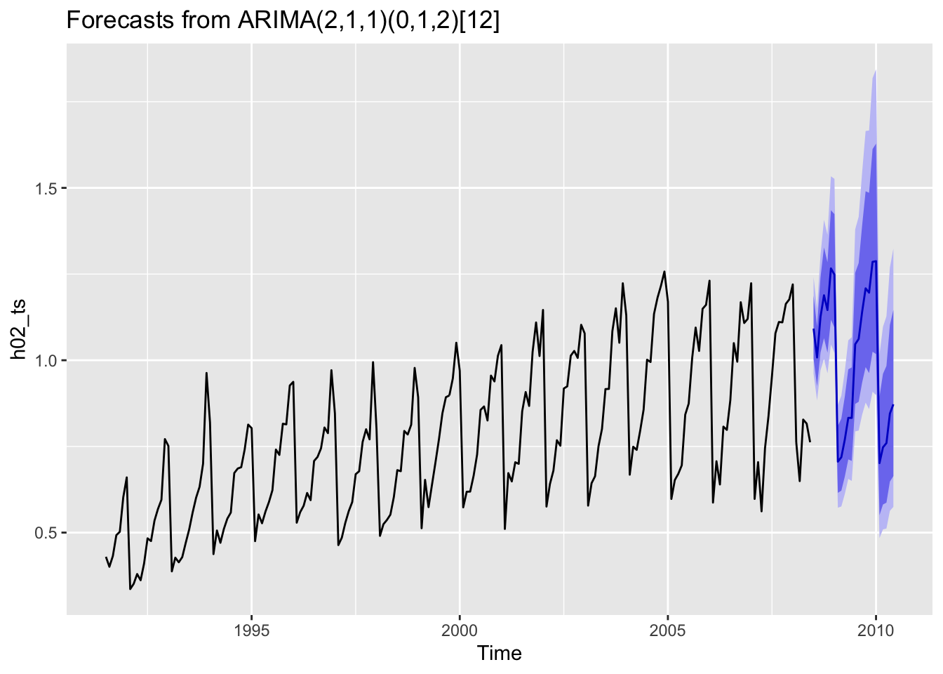
Although the auto-ARIMA algorithm chose a good model which accounts for the seasonality well, it does not always choose the best model. In fact, if analyzed thoroughly, an ARIMA(3,0,1)(0,1,2)[12] model has lower (i.e. better) RMSE and AICc values. For time series that are absolutely crucial, it may be worth the effort to manually choose a model by examining the ACF/PACF instead of relying completely on the auto-ARIMA algorithm.
7.2 fpp3 Method: Auto-ARIMA | Seasonal
The following example will utilize a dataset containing the quarterly European retail trade index from 1996-2011.
# 1. Plot the data and identify any unusual observations.
# 2. If the variance is unstable, then apply a transformation to stabilize it.
# 3. If the data are not stationary, then take a seasonal difference and/or regular difference until it is so.

# Convert ts to tsibble
eu_retail_tsbl <- fpp2::euretail %>% as_tsibble()

# Add seasonal + regular differencing, pivot long
eu_retail_tsbl_plot <- eu_retail_tsbl %>%
  transmute(
    `Trade Index` = value,
    `Annual Change in Index` = difference(value, lag=4),  # Quarterly = 4 lags
    `Double-Differenced Change in Index` = difference(value, lag=4) %>% difference()
  ) %>%
  gather("Type", "Sales", !!!syms(measured_vars(.)), factor_key=TRUE)

# Facet plot by Type
eu_retail_tsbl_plot %>%
  ggplot(aes(x=index, y=Sales)) +
  geom_line() +
  facet_grid(vars(Type), scales="free_y") +
  labs(title = "European retail trade index", x = "Quarter", y = "")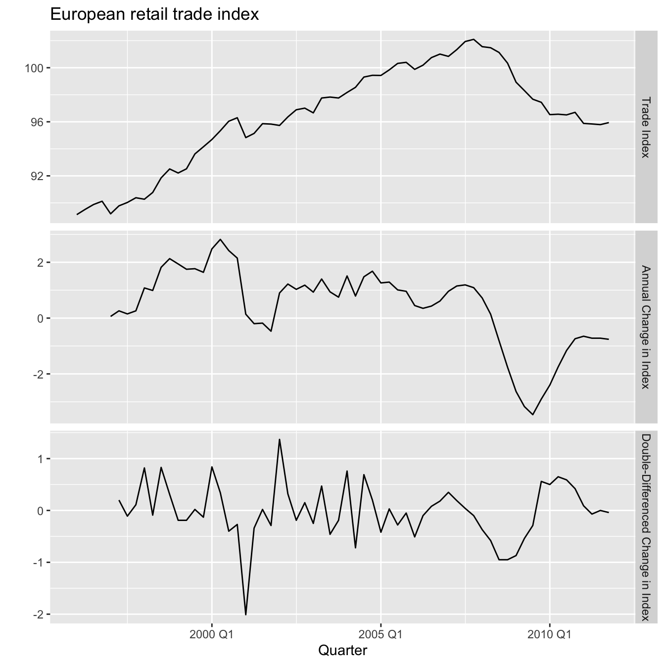
The first plot shows the original trade index series which is non-stationary as it shows a clear upwards then downwards trend as well as some seasonality. The second plot shows that the seasonally-differenced annual change in index series is still non-stationary showing an overall downward trend. The third plot shows that the seasonally-differenced and first-differenced change in index series is finally stationary. Let’s apply two different automatically chosen ARIMA models.
# 4a. Automatically fit multiple models and find the lowest AICc with approximation + stepwise approach.
fit_eu_retail_opt <- eu_retail_tsbl %>%
  model(
    `Auto-ARIMA Optimized` = ARIMA(value ~ index,
                                   stepwise = TRUE,
                                   approximation = TRUE))

# Check auto-ARIMA report
report(fit_eu_retail_opt)
## Series: value
## Model: LM w/ ARIMA(2,1,0)(1,1,1)[4] errors
##
## Coefficients:
## ar1 ar2 sar1 sma1 index
## 0.3507 0.2645 -0.0088 -0.8200 -0.1168
## s.e. 0.1361 0.1392 0.1855 0.1942 0.2075
##
## sigma^2 estimated as 0.291: log likelihood=-30.16
## AIC=72.31 AICc=73.93 BIC=84.78Will increasing the number of models to search for lead to a lower AICc score?
# 4b. Automatically fit multiple models and find the lowest AICc w/o approximation + stepwise approach.
fit_eu_retail_non_opt <- eu_retail_tsbl %>%
  model(
    `Auto-ARIMA Non-Optimized` = ARIMA(value ~ index,
                                       stepwise = FALSE,
                                       approximation = FALSE))

# Check auto-ARIMA report
report(fit_eu_retail_non_opt)
## Series: value
## Model: LM w/ ARIMA(0,1,3)(0,1,1)[4] errors
##
## Coefficients:
## ma1 ma2 ma3 sma1 index
## 0.2303 0.3760 0.4444 -0.6724 0.1095
## s.e. 0.1409 0.1177 0.1363 0.1564 0.2282
##
## sigma^2 estimated as 0.2354: log likelihood=-28.52
## AIC=69.03 AICc=70.65 BIC=81.5# Combine model metrics, sort by lowest AICc
auto_arima_metrics <- fit_eu_retail_opt %>%
glance() %>%
bind_rows(glance(fit_eu_retail_non_opt)) %>%
arrange(AICc)
# Show metrics summary
auto_arima_metrics## # A tibble: 2 x 8
## .model sigma2 log_lik AIC AICc BIC ar_roots ma_roots
## <chr> <dbl> <dbl> <dbl> <dbl> <dbl> <list> <list>
## 1 Auto-ARIMA Non-Optimized 0.235 -28.5 69.0 70.6 81.5 <cpl [0]> <cpl [7]>
## 2 Auto-ARIMA Optimized 0.291 -30.2 72.3 73.9 84.8 <cpl [6]> <cpl [4]>The
glance()function is useful for summarizing a model’s fit in a neattibbleformat. Setting thestepwiseandapproximationparameters toFALSEmeans the algorithm will test a much larger variety of ARIMA models. For this particular time series, doing this leads to a slightly lower AICc score. However, this process is computationally expensive and does not guarantee a better fitting model. In fact, an ARIMA(0,1,3)(0,1,1)[4] model which was manually chosen after examining the ACF & PACF shows an even lower AICc. Let’s see why this manually chosen model is a better fit and then apply it.
# Plot the double-differenced seasonal data with ACF & PACF
eu_retail_tsbl %>%
  gg_tsdisplay(
    value %>% difference(4) %>% difference(),
    plot_type = "partial"
    ) +
  ggtitle("Double-differenced Euro trade index")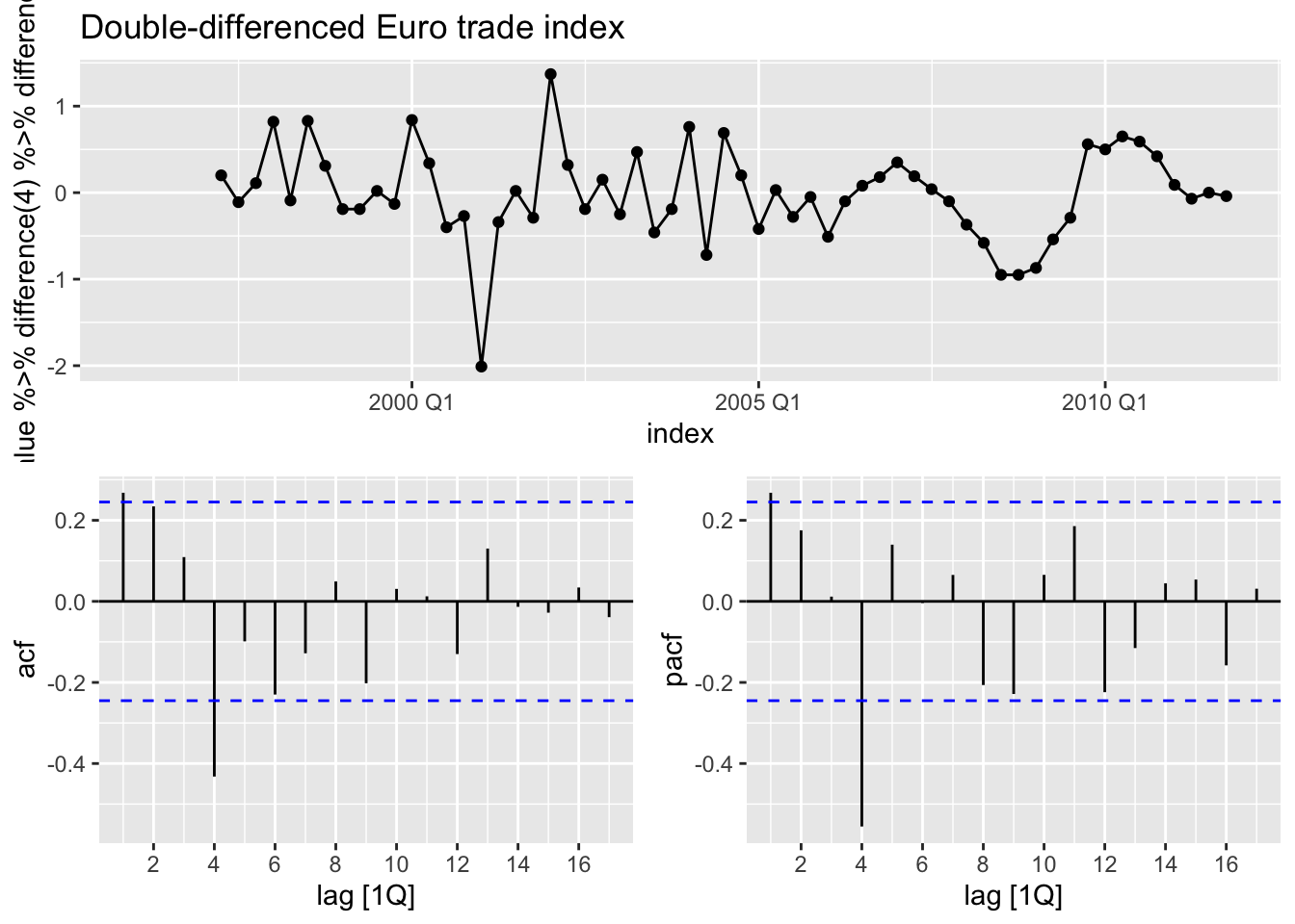
The significant spike at lag 1 in the ACF plot suggests a non-seasonal MA(1) component. Additionally, the significant spike at lag 4 in the ACF plot suggests a seasonal MA(1) component. Therefore an ARIMA(0,1,1)(0,1,1)[4] model (first and seasonal difference + non-seasonal and seasonal MA(1) components) would be a good place to start for testing models manually.
# Manually fit an ARIMA(0,1,1)(0,1,1)[4] model
fit_eu_retail_011_011 <- eu_retail_tsbl %>%
  model(ARIMA(value ~ pdq(0,1,1) + PDQ(0,1,1)))

# Check residuals
fit_eu_retail_011_011 %>%
  gg_tsresiduals() +
  ggtitle("Residuals from fitted ARIMA(0,1,1)(0,1,1)[4] model")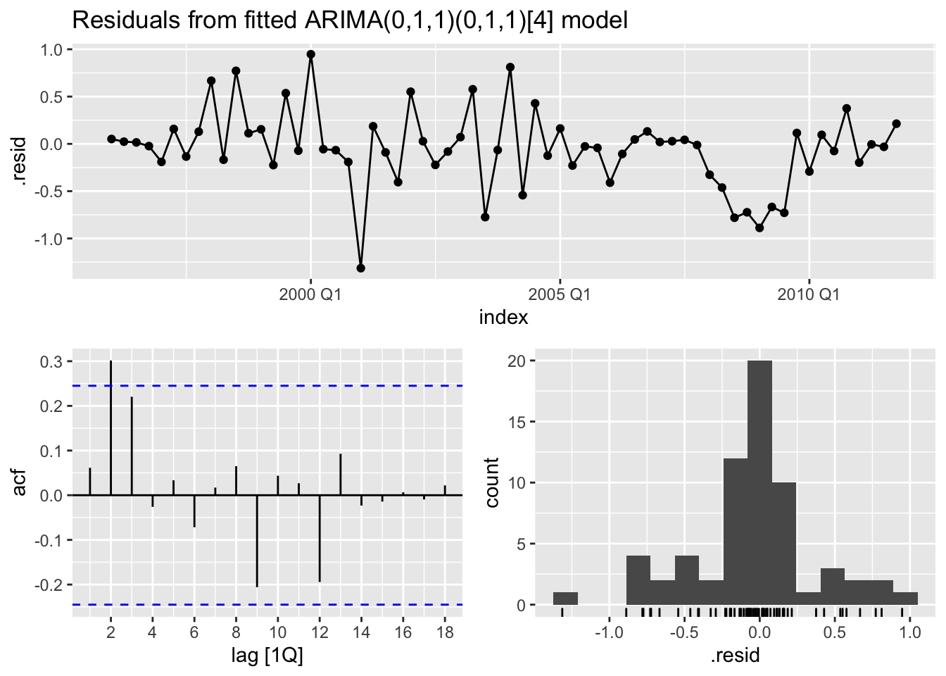
The ACF plot shows a significant spike at lag 2 and a fairly significant spike at lag 3. This suggests that more non-seasonal terms would result in a better model. At this point, adding an additional non-seasonal term step-by-step in a sequential fashion and then minimizing the AICc score would be a good plan of action. In this case, since we already know that an ARIMA(0,1,3)(0,1,1)[4] results in the lowest AICc, we’ll skip over analyzing an ARIMA(0,1,2)(0,1,1)[4] model for now.
# Manually fit an ARIMA(0,1,3)(0,1,1)[4] model
fit_eu_retail_013_011 <- eu_retail_tsbl %>%
  model(
    `ARIMA(0,1,3)(0,1,1)[4]` = ARIMA(value ~ pdq(0,1,3) + PDQ(0,1,1)))

# 5. Plot ACF of the residuals and do a portmanteau test to make sure they look like white noise.
fit_eu_retail_013_011 %>%
  gg_tsresiduals() +
  ggtitle("Residuals from fitted ARIMA(0,1,3)(0,1,1)[4] model")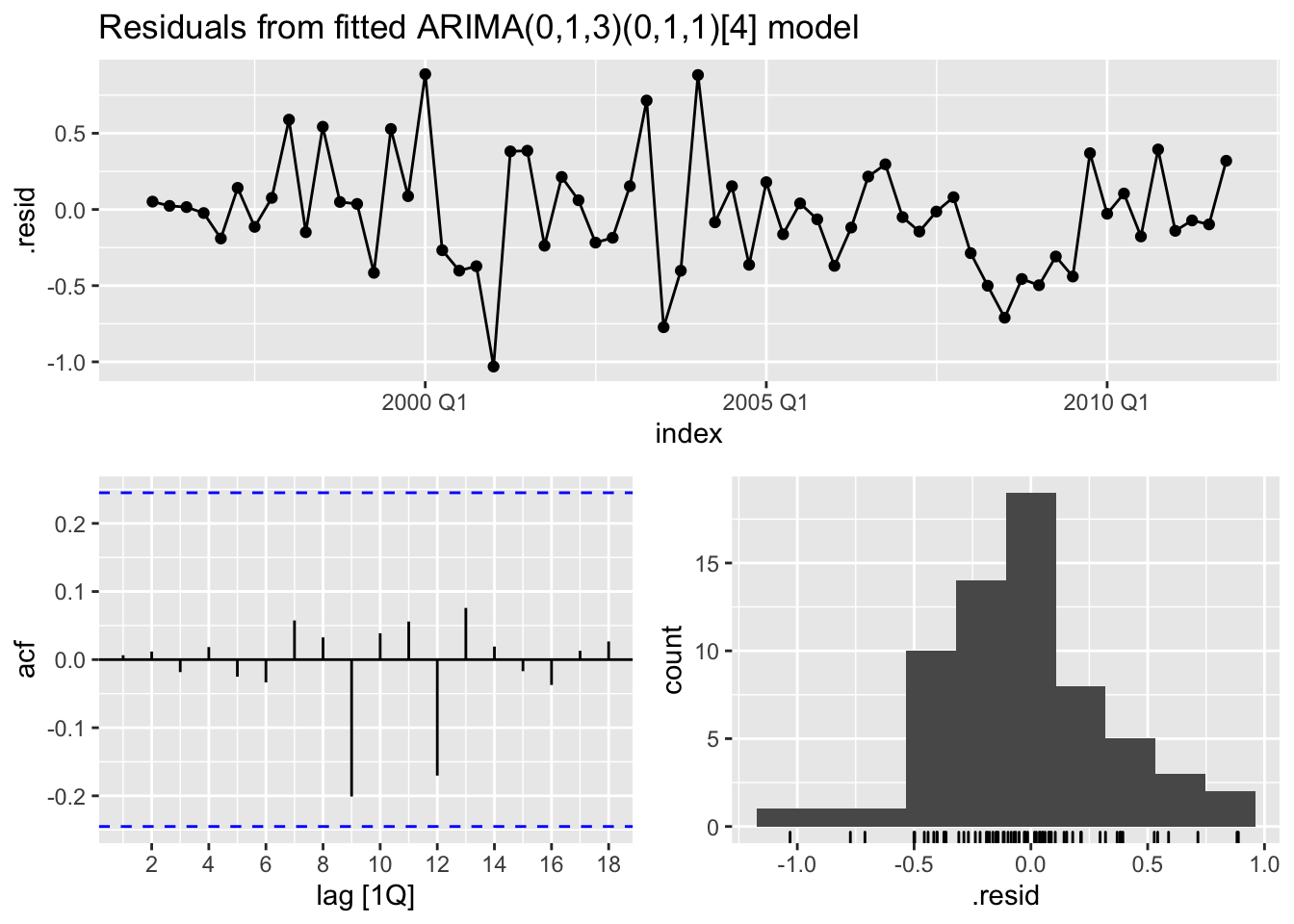
The residuals for an ARIMA(0,1,3)(0,1,1)[4] model shows all spikes within the significance limits in the ACF plot. This suggests that they are white noise. Now run a Ljung-Box test to make sure.
# Ljung-Box white noise test (p-value > 0.05)
fit_eu_retail_013_011 %>%
  augment() %>%
  select(.resid, index) %>%
  features(.resid, ljung_box, lag=20, dof=0) # Or use box_pierce instead
## # A tibble: 1 x 2
## lb_stat lb_pvalue
## <dbl> <dbl>
## 1 7.40 0.995The residuals for an ARIMA(0,1,3)(0,1,1)[4] model passes the Ljung-Box test as it confirms that they have no remaining autocorrelation with a p-value > 0.05. We can confidently say that the residuals are white noise. Now check the model report for the AICc.
# Check manual ARIMA report for AICc
fit_eu_retail_013_011 %>% report()
## Series: value
## Model: ARIMA(0,1,3)(0,1,1)[4]
##
## Coefficients:
## ma1 ma2 ma3 sma1
## 0.2630 0.3694 0.4200 -0.6636
## s.e. 0.1237 0.1255 0.1294 0.1545
##
## sigma^2 estimated as 0.156: log likelihood=-28.63
## AIC=67.26 AICc=68.39 BIC=77.65Let’s combine and compare the summary metrics for this manually chosen model to the two automatically chosen models just for fun.
# Combine auto-ARIMA + manual ARIMA metrics into tibble
auto_arima_metrics %>%
  bind_rows(fit_eu_retail_013_011 %>% glance()) %>%
  arrange(AICc)
## # A tibble: 3 x 8
## .model sigma2 log_lik AIC AICc BIC ar_roots ma_roots
## <chr> <dbl> <dbl> <dbl> <dbl> <dbl> <list> <list>
## 1 ARIMA(0,1,3)(0,1,1)[4] 0.156 -28.6 67.3 68.4 77.6 <cpl [0]> <cpl [7]>
## 2 Auto-ARIMA Non-Optimized 0.235 -28.5 69.0 70.6 81.5 <cpl [0]> <cpl [7]>
## 3 Auto-ARIMA Optimized 0.291 -30.2 72.3 73.9 84.8 <cpl [6]> <cpl [4]>The AICc of the manually chosen ARIMA model is lower than the automatically chosen models. Now it’s finally time to plot some forecasts using the best model.
# Plot 3-year forecasts
fit_eu_retail_013_011 %>%
  forecast(h = 12) %>% # 3 years = 12 quarters
  autoplot(eu_retail_tsbl) +
  labs(
    title="European retail trade index 3-year forecast",
    subtitle="ARIMA(0,1,3)(0,1,1)[4] model",
       x="Quarter", y="Trade Index")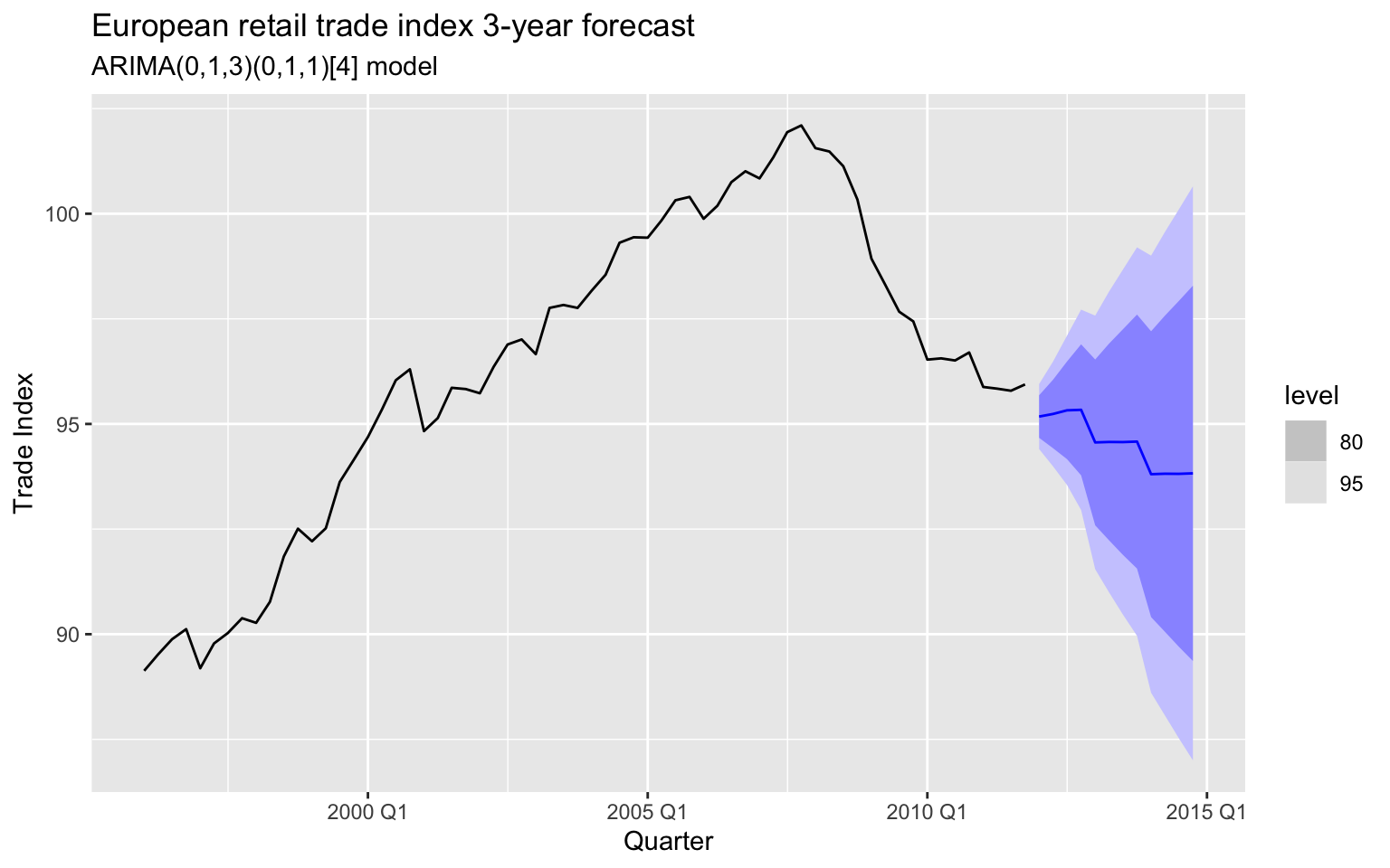
By double-differencing the data, the 3-year forecasts follows the recent downwards trend. The large prediction intervals allow for the data to trend upwards even though the point forecast trends downwards. The main point of all this is to illustrate that relying on an algorithm to automatically select an ARIMA model will not always give the best fitting model. As the saying goes: if you want a job well done, sometimes you gotta do it yourself.
7.3 modeltime Method: Auto-ARIMA | Seasonal
The following example will utilize a dataset containing the total US monthly job numbers in various industries but will focus on the leisure and hospitality industry from 2000-2019.
# 1. Plot the data and identify any unusual observations.

# Filter the data, convert tsibble to tibble
leisure_tbl <- us_employment %>%
  filter(
    Title == "Leisure and Hospitality",
    year(Month) > 2000
    ) %>%
  mutate(
    Employed = Employed / 1000,  # In millions
    Month = as_date(Month)
    ) %>%
  select(Month, Employed) %>%
  tk_tbl(preserve_index = FALSE)

leisure_tbl %>%
  plot_time_series(
    .date_var = Month,
    .value = Employed,
    .interactive = FALSE,
    .title = "Monthly employment in the US leisure & hospitality industry",
    .x_lab = "Month",
    .y_lab = "Jobs (In Millions)"
  ) +
  labs(subtitle = "1/2000 - 6/2019")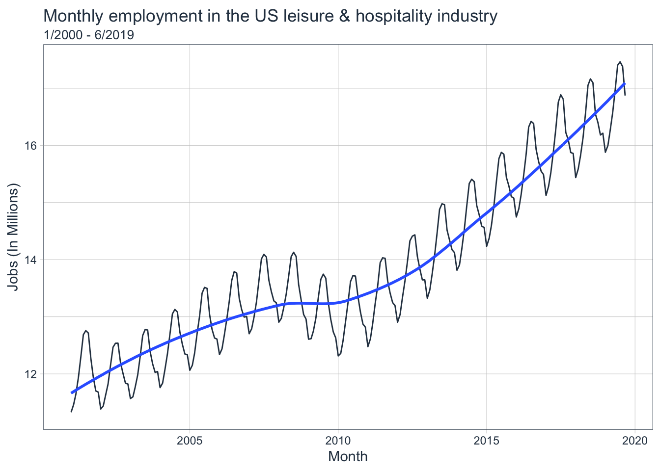
This time series is non-stationary with a clear seasonal pattern and non-linear trend. Since the variance is not increasing with the level, a transformation is not necessary so skip step 2. Let’s apply a seasonal difference and see what happens to the stationarity.
# 3. If the data are not stationary, then take a seasonal difference and/or a first difference until it is so.

# Add a column of seasonally differenced data
leisure_sd_tbl <- leisure_tbl %>%
  tk_augment_differences(
    .value = Employed,
    .lags = 12,
    .differences = 1
  )

# Plot seasonally-differenced data
leisure_sd_tbl %>%
  plot_time_series(
    .date_var = Month,
    .value = Employed_lag12_diff1, # Seasonally differenced data
    .interactive = FALSE,
    .title = "Monthly employment in the US leisure & hospitality industry",
    .x_lab = "Month",
    .y_lab = "Seasonally Differenced"
  ) +
  labs(subtitle = "1/2000 - 6/2019")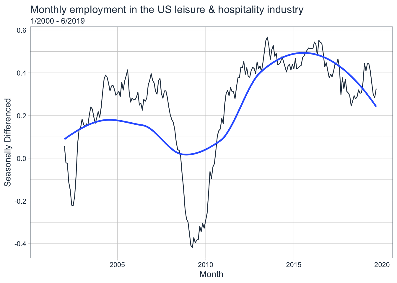
After applying a seasonal difference, the series is still not stationary. Let’s apply a first difference to this seasonally differenced data to make it stationary.
# Apply a first difference
leisure_sd_diff_tbl <- leisure_sd_tbl %>%
  tk_augment_differences(
    .value = Employed_lag12_diff1,
    .lags = 1,
    .differences = 1
  )

# Check that differencing was applied
leisure_sd_diff_tbl %>% tail()
## # A tibble: 6 x 4
## Month Employed Employed_lag12_diff1 Employed_lag12_diff1_lag1_diff1
## <date> <dbl> <dbl> <dbl>
## 1 2019-04-01 16.6 0.443 0.00100
## 2 2019-05-01 17.0 0.409 -0.0340
## 3 2019-06-01 17.4 0.352 -0.0570
## 4 2019-07-01 17.5 0.299 -0.053
## 5 2019-08-01 17.4 0.284 -0.015
## 6 2019-09-01 16.9 0.326 0.042Make sure to apply the first difference to the already seasonally-differenced data. Now check if the series is stationary and if so, plot the lag diagnostics.
# Plot seasonally + first differenced data
lh1 <- leisure_sd_diff_tbl %>%
  plot_time_series(
    .date_var = Month,
    .value = Employed_lag12_diff1_lag1_diff1, # Seasonal + first differenced data
    .interactive = FALSE,
    .title = "Monthly employment in the US leisure & hospitality industry from 2000-2019",
    .x_lab = "Month",
    .y_lab = "Seasonally + First Differenced"
  )

# Plot lag diagnostics of seasonally + first differenced data
lh2 <- leisure_sd_diff_tbl %>%
  plot_acf_diagnostics(
    .date_var = Month,
    .value = Employed_lag12_diff1_lag1_diff1,
    .lags = 36,
    .interactive = FALSE,
    .show_white_noise_bars = TRUE
  )

# Arrange plots
plot_grid(lh1, lh2, ncol = 1, rel_heights = c(1, 2))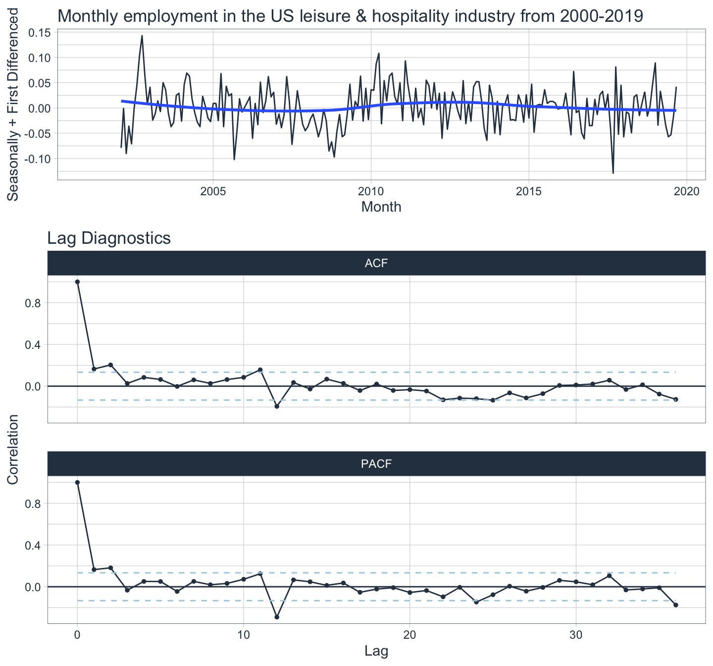
The series finally looks stationary after applying a seasonal difference and a first difference. There are significant spikes at lag 2 and lag 12 in the ACF plot which suggest a non-seasonal MA(2) component and seasonal MA(1) component respectively. A breakdown of all the components is as follows: first difference (d=1), seasonal difference (D=1), non-seasonal MA(2) (q=2), and seasonal MA(1) component (Q=1). We can summarize this as an ARIMA(0,1,2)(0,1,1)[12] model. It’s also possible to manually select an ARIMA by using the PACF to choose the non-seasonal aspect and the ACF to select the seasonal aspect of the model which would suggest an ARIMA(2,1,0)(0,1,1)[12] model. Let’s apply these two manually chosen models and an automatically chosen model and see what happens.
# 3. Automatically fit multiple models and find the lowest AICc.

# Split the data 80/20 into a training and test set
splits <- rsample::initial_time_split(leisure_tbl, prop = 0.8)

# Manually fit an ARIMA(0,1,2)(0,1,1)[12] model
model_fit_arima_012_011 <- arima_reg(
  non_seasonal_ar          = 0,  # p
  non_seasonal_differences = 1,  # d
  non_seasonal_ma          = 2,  # q
  seasonal_ar              = 0,  # P
  seasonal_differences     = 1,  # D
  seasonal_ma              = 1,  # Q
  seasonal_period          = 12  # Monthly data
  ) %>%
  set_engine("arima") %>%
  fit(Employed ~ Month, data = training(splits))

# Manually fit an ARIMA(2,1,0)(0,1,1)[12] model
model_fit_arima_210_011 <- arima_reg(
  non_seasonal_ar          = 2,  # p
  non_seasonal_differences = 1,  # d
  non_seasonal_ma          = 0,  # q
  seasonal_ar              = 0,  # P
  seasonal_differences     = 1,  # D
  seasonal_ma              = 1,  # Q
  seasonal_period          = 12  # Monthly data
  ) %>%
  set_engine("arima")%>%
  fit(Employed ~ Month, data = training(splits))

# Automatically fit an ARIMA model
model_fit_auto_arima <- arima_reg() %>%
  set_engine("auto_arima")%>%
  fit(Employed ~ Month, data = training(splits))
## frequency = 12 observations per 1 year# Add fitted models to a modeltime table
arima_models_tbl <- modeltime_table(
model_fit_arima_012_011,
model_fit_arima_210_011,
model_fit_auto_arima)
# Check modeltime table
arima_models_tbl## # Modeltime Table
## # A tibble: 3 x 3
## .model_id .model .model_desc
## <int> <list> <chr>
## 1 1 <fit[+]> ARIMA(0,1,2)(0,1,1)[12]
## 2 2 <fit[+]> ARIMA(2,1,0)(0,1,1)[12]
## 3 3 <fit[+]> ARIMA(2,1,1)(1,1,2)[12]Now that all the models have been fitted, best practices tell us to test each model’s residuals for white noise. However, since that process has already been shown in a previous example, we will skip step 4 here. The next step is to calibrate the fitted models on the test set to create confidence intervals and accuracy metrics. Note that calibration data are forecasting predictions and residuals calculated from out-of-sample data.
# Calibrate the model to produce confidence intervals
arima_models_calibration_tbl <- arima_models_tbl %>%
  modeltime_calibrate(new_data = rsample::testing(splits))

# Visualize the forecasts on the test set
arima_models_calibration_tbl %>%
  modeltime_forecast(
    new_data = testing(splits),
    actual_data =  leisure_tbl
  ) %>%
  plot_modeltime_forecast(
    .legend_max_width = 25,
    .interactive = TRUE,
    .title = "Visualizing ARIMA model forecasts on test set",
    .x_lab = "Month",
    .y_lab = "Jobs (In Millions)"
  ) %>%
  plotly::layout(  # Custom ggplotly layout
    legend = list(
      orientation = "h",
      xanchor = "center",
      x = 0.5,
      y = -0.2)
    )
Of interest is that all three models do well at capturing the seasonal pattern and the increasing trend extends the recent pattern as well. Instead of relying on the AICc,
modeltimeevaluates accuracy on the test (i.e. out-of-sample) set. Now decide which model fits the best based on various accuracy metrics.
# Check accuracy metrics
arima_models_calibration_tbl %>%
  modeltime_accuracy() %>%
  table_modeltime_accuracy(  # Fancy table
    .interactive = FALSE
)| Accuracy Table | ||||||||
|---|---|---|---|---|---|---|---|---|
| .model_id | .model_desc | .type | mae | mape | mase | smape | rmse | rsq |
| 1 | ARIMA(0,1,2)(0,1,1)[12] | Test | 0.10 | 0.62 | 0.39 | 0.61 | 0.13 | 0.98 |
| 2 | ARIMA(2,1,0)(0,1,1)[12] | Test | 0.11 | 0.66 | 0.42 | 0.66 | 0.14 | 0.98 |
| 3 | ARIMA(2,1,1)(1,1,2)[12] | Test | 0.06 | 0.38 | 0.24 | 0.38 | 0.08 | 0.99 |
The clear winner is model 3 which is the automatically chosen ARIMA model. It has better error metrics (lower is better) and even has a very slightly higher R-squared value (higher is better). Now refit the models to the full dataset and make future forecasts.
# Refit models to full dataset and forecast forward
arima_models_refit_tbl <- arima_models_calibration_tbl %>%
  # filter(.model_id == 3) %>%  # Only show best model
  modeltime_refit(data = leisure_tbl)

# Plot 3-year forecasts
arima_models_refit_tbl %>%
  modeltime_forecast(
    h = "3 years",
    actual_data = leisure_tbl
  ) %>%
  plot_modeltime_forecast(
    .legend_max_width = 25,
    .interactive = TRUE,
    .title = "Monthly employment in the US leisure & hospitality industry w/ 3-year forecasts",
    .x_lab = "Month",
    .y_lab = "Jobs (In Millions)"
  ) %>%
  plotly::layout(
    title = list(
      text = paste0("Monthly employment in the US leisure & hospitality industry",
                    "<br>",
                    "<sup>",
                    "3-year forecasts starting from October 2019",
                    "</sup>")),
    legend = list(
      orientation = "h",
      xanchor = "center",
      x = 0.5,
      y = -0.2))
“Complex inventions can make your life simple.” - The Grouch, Lyrics to “No More Greener Grasses.”
8. Conclusions about ARIMA models
ARIMA and ETS models are some of the most widely used forecasting techniques. They are complementary to each other: ARIMA models focus on the autocorrelations in the data whereas ETS models focus on the trend and seasonality.
Here are some of my thoughts about ARIMA models:
- Visualizing and identifying different patterns in your time series data is always the first step in forecasting.
- The Hyndman-Khandakar algorithm for automatic ARIMA modeling does not always choose a model with the best AICc score.
- A model with the best AICc that was fit on a training set may not be the best model when fitting on a test set.
- Just because the residuals of a model do not pass every test for white noise does not mean the model is unsuitable for forecasting; it is certainly possible that the best-performing model will fail a test or two.
Here are some of my thoughts about the three forecasting frameworks utilized in this article:
fpp2is considered to be outdated and is no longer maintained;fpp3andmodeltime+timetkare currently maintained.- The
fpp2andfpp3frameworks focus more on minimizing the AICc for ARIMA model selection whereasmodeltime+timetkfocuses more on accuracy measures on an out-of-sample test set. - All three frameworks
fpp2,fpp3, andmodeltime+timetkrely on theforecastpackage and thus will give similar results; however, they all have different methodologies with their own respective strengths and weaknesses.
Every forecaster should at least consider trying ETS and ARIMA models before jumping to more complex methods like machine-learning and neural networks. This is especially true in situations where you are forecasting with univariate data and where scaling to many time series is an issue.